Part 4 of 6 in the Technical Series: Emergency Pressure Relief & Effluent Handling Systems

# Runaway Reactions & Calorimetry for Emergency Vent Sizing (Part 4)

Chemical runaway reactions present the most violent, high-consequence process safety hazard in batch synthesis, specialty polymers, agrochemicals, and active pharmaceutical ingredient (API) manufacturing. Unlike conventional mechanical or operational upsets—such as an external pool fire, blocked pump discharge, or tube rupture—an uncontrolled exothermic reaction generates heat internally within the bulk liquid phase. Because reaction rates accelerate exponentially with temperature according to the Arrhenius law, the volumetric rate of heat release rapidly outstrips the heat removal capability of reactor jackets or external circulation coolers.

If emergency pressure relief systems are not engineered using rigorous DIERS (Design Institute for Emergency Relief Systems) methodology, the internal pressure will surge beyond the ultimate tensile strength of the vessel shell, culminating in catastrophic brittle or ductile rupture, blast overpressure waves, structural collapse, and toxic vapor cloud dispersion.

This comprehensive technical masterclass provides process safety and chemical engineers with the complete mathematical and experimental framework required to:

1. Accurately diagnose and classify reactive systems into Tempered (Vapor), Gassy, or Hybrid regimes using thermodynamic pressure-temperature ($P-T$) response curves and Clausius-Clapeyron analysis.
2. Interpret and scale raw data from modern adiabatic reaction calorimeters (ARC, ARSST, and VSP2), correcting for thermal inertia ($\phi$-factor) and extracting kinetic parameters ($T_{onset}$, $(dT/dt)_{max}$, $(dP/dt)_{max}$, $TMR_{ad}$).
3. Quantify reactor hydrodynamics and two-phase level swell, distinguishing between churn-turbulent and foamy bubbly regimes using the Zuber-Findlay drift-flux model.
4. Size emergency relief systems using validated analytical models: the Fauske direct equation, the Leung saturated tempered model, the Leung gassy equation, and hybrid volumetric formulations.
5. Review three complete numerical worked engineering examples covering tempered polymerizations, gassy peroxide decompositions, and hybrid nitrations.

# 1. The Physics and Kinetics of Thermal Runaways

The mathematical foundation of runaway exotherms is governed by Semenov thermal explosion theory, which balances non-linear Arrhenius heat generation against linear Newtonian cooling across the vessel boundary:

Where:

• $V$ = Liquid reaction volume ($\text{m}^3$)
• $-\Delta H_{rxn}$ = Exothermic heat of reaction ($\text{J/mol}$)
• $A$ = Pre-exponential frequency factor ($\text{s}^{-1}$ or $\text{m}^3/(\text{mol}\cdot\text{s})$)
• $C_A$ = Reactant concentration ($\text{mol/m}^3$), with reaction order $n$
• $E_a$ = Apparent activation energy ($\text{J/mol}$)
• $R$ = Universal gas constant ($8.3144 \text{ J}/(\text{mol}\cdot\text{K})$)
• $T$ = Bulk reacting liquid temperature ($\text{K}$)
• $U$ = Overall heat transfer coefficient ($\text{W}/(\text{m}^2\cdot\text{K})$)
• $A_{jacket}$ = Wetted heat transfer area ($\text{m}^2$)
• $T_{jacket}$ = Cooling jacket coolant temperature ($\text{K}$)

graph TD
    A["Cooling Jacket Failure / Agitation Loss / Wrong Catalyst Charge"] --> B["Reactor Temperature Rises: T > T_critical"]
    B --> C["Arrhenius Heat Rate Acceleration: Q_gen proportional to exp(-Ea / RT)"]
    C --> D["Exponential Divergence: Q_gen >> Q_rem (Self-Heating)"]
    D --> E{"Thermodynamic Classification of Mass"}
    E -->|Tempered System: Volatile Solvent| F["Evaporative Latent Heat Boiling Limits Peak Temperature"]
    E -->|Gassy System: Non-Condensable Gas| G["Decomposition Produces Gas: Zero Latent Heat Cooling!"]
    E -->|Hybrid System: Gas + Solvent Vapor| H["Simultaneous Permanent Gas Generation & Solvent Boiling"]
    F --> I["DIERS Two-Phase Sizing: Fauske / Leung Vapor Models"]
    G --> J["DIERS Gas / Two-Phase Foamy Sizing: Leung Gassy Model"]
    H --> K["DIERS Hybrid Sizing: Dual-Contribution Volumetric Model"]

# Critical Runaway Parameters:

• Adiabatic Temperature Rise ($\Delta T_{ad}$): The maximum possible temperature elevation assuming zero heat dissipation to the vessel surroundings:

• Time to Maximum Rate under Adiabatic Conditions ($TMR_{ad}$): The operational escape time available between the initial self-heating detection and peak reaction velocity. For a zero-order or early-stage runaway:

Where $q_0 = C_p (dT/dt)_0$ is the specific heat generation rate at the initial temperature $T_0$.

• Self-Accelerating Decomposition Temperature (SADT): The lowest ambient temperature at which a packaged chemical substance or bulk storage tank undergoes runaway self-heating within a period of one week.
• Frank-Kamenetskii vs. Semenov Regimes: In well-agitated liquid batch reactors with low viscosity, the Biot number is low ($Bi = h L / k < 0.1$), and the Semenov lumped parameter model holds (uniform temperature throughout the liquid). In high-viscosity polymer melts, stagnant unstirred tanks, or solid powder beds, internal conduction resistance dominates, creating hot spots governed by the Frank-Kamenetskii distributed parameter model.

# 2. Thermodynamic System Identification: Tempered, Gassy, and Hybrid Systems

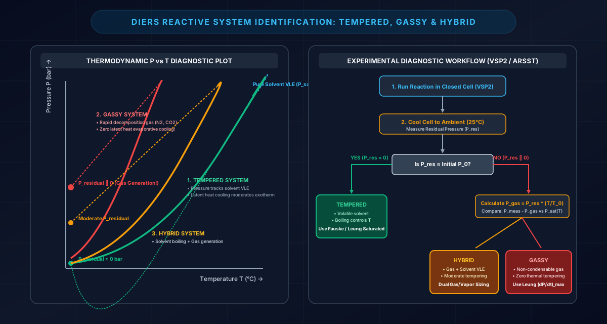
Correctly identifying whether a chemical reaction system is Tempered, Gassy, or Hybrid is the absolute first step in emergency relief sizing. An error in classification will lead to catastrophically undersized relief equipment.

# Diagnostic Distinction Criteria

# 1. Tempered (Vapor) Systems

• Physical Mechanism: The reacting liquid contains a volatile solvent or reactant in vapor-liquid equilibrium (VLE). When the reactor relief device opens, the liquid flashes and boils. The latent heat of vaporization ($\Delta H_v$) carries heat away from the reacting mass at a rate of $\dot{Q}_{evap} = \dot{m}_{evap} \Delta H_v$. This evaporative cooling tempers (quenches or holds) the reaction temperature at the boiling point corresponding to the vessel relief pressure.
• Calorimeter P-T Behavior: In a closed adiabatic test cell (VSP2 or ARC), the total pressure tracks the saturated vapor pressure curve of the solvent exactly:

A plot of $\ln P$ vs. $-1/T$ (Clausius-Clapeyron coordinate) yields a straight line with slope $-\Delta H_v / R$.

• Cooling Behavior: When the calorimeter heater is switched off and the test cell cools back to ambient temperature ($25^\circ\text{C}$), the pressure drops back down to the baseline vapor pressure. Residual non-condensable gas pressure is negligible ($P_{residual} \approx 0 \text{ bar(g)}$).
• Industrial Examples:
  • Free radical polymerization of styrene or butyl acrylate in ethylbenzene/toluene.
  • Grignard reagent synthesis in tetrahydrofuran (THF) or diethyl ether.
  • Friedel-Crafts alkylation of aromatics in hexane or dichloromethane.

# 2. Gassy Systems

• Physical Mechanism: The reaction is a chemical decomposition that releases permanent, non-condensable gases (such as $N_2, CO_2, CO, O_2, H_2, CH_4$) in the absence of an evaporating volatile liquid. Because permanent gases do not condense at reactor operating temperatures and undergo no phase change, venting gas removes mass from the reactor but provides zero latent heat cooling!
• Calorimeter P-T Behavior: Pressure builds up rapidly as gas moles accumulate ($P = n_g R T / V_{headspace}$). The rate of pressure rise $(dP/dt)$ is directly proportional to chemical kinetic reaction velocity, not temperature alone. On a $\ln P$ vs. $-1/T$ plot, the trajectory curves upward steeply and erratically, diverging completely from the Clausius-Clapeyron vapor pressure relationship.
• Cooling Behavior: When the test cell is cooled back to $25^\circ\text{C}$, the generated gas remains in the gas phase. A massive residual pressure ($P_{residual} \gg 0$, often $20 \text{ to } 150 \text{ bar}$) remains in the bomb.
• Industrial Examples:
  • Thermal decomposition of organic peroxides (e.g., tert-butyl peroxybenzoate, MEKP, dicumyl peroxide).
  • Diazonium salt couplings releasing stoichiometric $N_2$ gas.
  • Catalytic decomposition of concentrated hydrogen peroxide ($H_2O_2 \to H_2O + \frac{1}{2} O_2$).
  • Self-accelerating decomposition of hydroxylamine or nitro-compounds.

# 3. Hybrid Systems

• Physical Mechanism: Both phenomena occur simultaneously. The reaction generates significant quantities of permanent non-condensable gases while operating in the presence of a volatile liquid solvent that exerts substantial vapor pressure.
• Calorimeter P-T Behavior: Total measured pressure is the sum of solvent vapor pressure and partial pressure of generated gas:

During early runaway, solvent vapor pressure dominates; as kinetic rates accelerate, gas generation drives the curve upward above the pure solvent VLE curve.

• Cooling Behavior: Upon cooling back to ambient temperature, the solvent condenses back into liquid, but the non-condensable gas creates a moderate residual pressure ($P_{residual} > 0$, typically $2 \text{ to } 20 \text{ bar}$).
• Industrial Examples:
  • Mixed-acid aromatic nitrations (nitration of toluene to dinitrotoluene, generating $NO_x$ gas byproducts while boiling nitric acid and water).
  • Acid-catalyzed phenolic resin condensation (generating gaseous side products alongside steam).
  • Sulfonation reactions releasing gaseous $SO_2$ alongside boiling volatile organics.

# Summary Diagnostic Matrix

# 3. Calorimetric Instruments & Experimental Data Interpretation

Accurate reactive vent design depends entirely on obtaining high-fidelity experimental data under adiabatic conditions. Standard analytical tools like Differential Scanning Calorimetry (DSC) test milligram quantities in closed micro-crucibles; they cannot measure pressurization rates, cannot track two-phase foaming swell, and cannot simulate plant-scale thermal dynamics.

# Comparison of Industrial Adiabatic Calorimeters

# 1. ARC (Accelerating Rate Calorimeter)

• Design: Employs a spherical, heavy-walled metal bomb ($10 \text{ mL}$) made of titanium, Hastelloy C, or stainless steel inside a radiant spherical heater jacket.
• Operational Mode: Heat-Wait-Search (HWS). The instrument steps temperature in $5^\circ\text{C}$ increments, waits for thermal equilibrium, and searches for self-heating above a sensitive threshold ($\ge 0.02 \text{ K/min}$).
• Strengths: Unrivaled sensitivity for pinpointing the absolute earliest thermal onset temperature ($T_{onset}$) and calculating true zero-order kinetic parameters ($E_a, A$).
• Limitations: The heavy metallic bomb absorbs a large fraction of the reaction heat, creating a high thermal inertia ($\phi \approx 1.5 - 3.0$). Furthermore, pressure containment limits ($< 150 \text{ bar}$) prevent testing high-rate decompositions, and open-cell blowdown venting cannot be performed.

# 2. VSP2 (Vent Sizing Package 2)

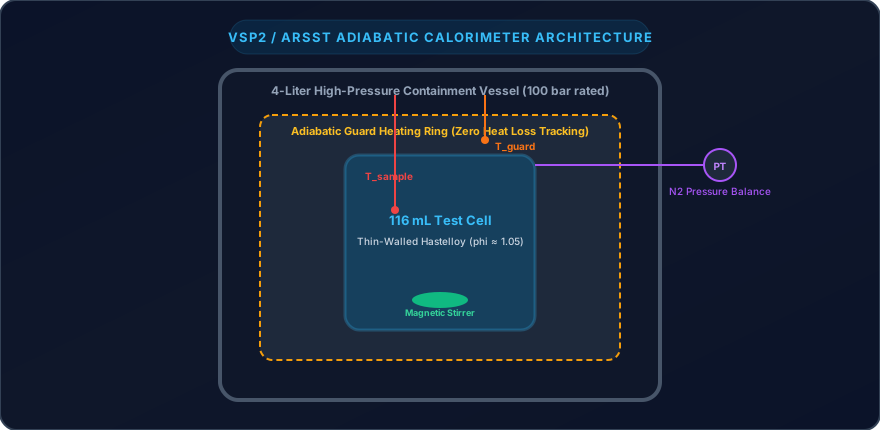
• Design: Developed specifically under the AIChE DIERS project for emergency vent sizing. Uses an ultra-thin-walled test cell ($116 \text{ mL}$, wall thickness $0.15 \text{ mm}$) housed inside a $4 \text{ L}$ heavy-duty containment vessel.
• Operational Mode: An active nitrogen tracking system pressurizes the containment vessel to match the internal test cell pressure in real time ($\Delta P_{wall} \approx 0$). This eliminates mechanical stress on the test cell, allowing the cell mass to be minimal.
• Strengths: Achieves $\phi \approx 1.05 - 1.10$, virtually identical to a full-scale plant reactor! Capable of magnetic high-shear stirring, bottom liquid/gas injection, and direct open-cell blowdown tests to observe two-phase level swell directly.

# 3. ARSST (Advanced Reactive System Screening Tool)

• Design: Uses an open or loosely capped glass test cell ($10 \text{ mL}$) fitted with a low thermal mass heating coil inside a $350 \text{ mL}$ pressure vessel.
• Operational Mode: Operated under a constant low power heating rate ($0.5 \text{ to } 2.0 \text{ K/min}$) or pseudo-adiabatic mode. The vessel is pre-pressurized with $20 \text{ to } 30 \text{ bar}$ of nitrogen to suppress solvent boiling and evaluate gassy behavior directly.
• Strengths: Low cost, rapid testing turnaround (several tests per day), ultra-low thermal inertia ($\phi \approx 1.04$), and safe testing of highly energetic materials.

# Step-by-Step Protocol: Converting Calorimeter Data into Relief Vent Calculations

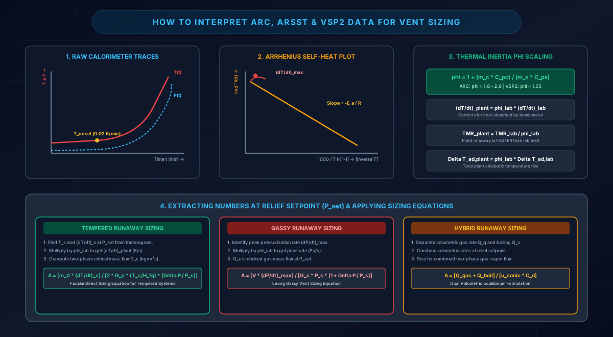
To take raw experimental data from an ARC, ARSST, or VSP2 test and apply it directly to emergency vent sizing equations, follow this rigorous 5-step engineering protocol:

# Step 1: Extract Raw Thermograms

Extract the time-dependent temperature $T(t)$ and pressure $P(t)$ data files. Identify:

• Onset Temperature ($T_{onset}$): The temperature where self-heating rate exceeds the instrument threshold ($0.02 \text{ K/min}$ for ARC, $0.1 \text{ K/min}$ for VSP2).
• Maximum Observed Temperature ($T_{max,obs}$) and Maximum Observed Pressure ($P_{max,obs}$).

# Step 2: Calculate Derivatives and Construct Arrhenius Plots

Perform numerical differentiation on the $T(t)$ and $P(t)$ time-series data:

Plot $\ln(dT/dt)_{lab}$ vs. $1000/T$ (Arrhenius coordinate). The linear slope in the early runaway region yields the activation energy:

# Step 3: Apply Thermal Inertia ($\phi$-Factor) Scale-Up Correction

In a laboratory calorimeter, a portion of the heat of reaction is absorbed by the metallic cell wall rather than heating the chemical sample. The thermal inertia factor ($\phi$) is defined as:

• In a laboratory ARC: $\phi_{lab} \approx 1.5 - 2.8$.
• In a laboratory VSP2: $\phi_{lab} \approx 1.05 - 1.10$.
• In a commercial $10 \text{ m}^3$ plant reactor: $\phi_{plant} \approx 1.01 - 1.03$ (the metal wall mass is negligible compared to tens of tons of liquid).

Because thermal inertia artificially depresses self-heat and pressurization rates, the laboratory data must be scaled up to plant conditions:

# Step 4: Calculate Time to Maximum Rate ($TMR_{ad}$)

Integrate the corrected self-heat curve backwards from peak velocity to evaluate operator intervention response windows:

If $TMR_{ad} < 30 \text{ minutes}$, automated emergency relief or automated emergency quenching is mandatory; human manual intervention cannot be credited.

# Step 5: Select the Relief Design Setpoint

• Establish the relief device set pressure $P_{set} \le P_{MAWP}$.
• Establish the maximum allowable accumulated relieving pressure:

(Typically $10\%$ overpressure for ASME single-device protection, or $16-21\%$ for multiple devices or fire scenarios).

• For a Tempered System: Find the temperature $T_s$ corresponding to saturation vapor pressure $P_s$, and read the corrected self-heat rate $(dT/dt)_s$ at $T_s$.
• For a Gassy System: Locate the point of maximum reaction velocity and read the peak pressurization rate $(dP/dt)_{max,plant}$.
• For a Hybrid System: Extract both $(dT/dt)_s$ and the gas generation rate $(dn_g/dt)_s$ at the relieving setpoint.

# 4. Reactor Hydrodynamics & Two-Phase Level Swell

When an emergency vent opens on a boiling or gas-generating runaway reactor, vapor bubbles nucleate throughout the liquid mass. As bubbles rise, they drag liquid upward, causing the liquid surface to swell (level swell). If the expanded two-phase foam or bubbly surface reaches the top relief nozzle, the discharged fluid transitions from single-phase vapor/gas to two-phase liquid-vapor mixture.

graph TD
    Bubble["Gas / Vapor Bubbles Form Throughout Reacting Liquid"] --> Visc{"Fluid Chemistry & Foaming Tendency"}
    
    Visc -->|Low Viscosity, Non-Foaming, Pure Solvents| Churn["CHURN-TURBULENT FLOW REGIME"]
    Visc -->|Foaming Liquids, Viscous Resins (mu > 50 cP), Surfactants| Bubbly["BUBBLY / FOAMY HOMOGENEOUS REGIME"]
    
    Churn --> Dis1["Rapid Bubble Coalescence: High Slip Velocity u_inf"]
    Dis1 --> Cut1["Surface Disengages: Pure Vapor Relief When Liquid Drops < 40-50%"]
    
    Bubbly --> Dis2["Bubbles Entrained in Viscous Liquid Matrix: Zero Slip"]
    Dis2 --> Cut2["HOMOGENEOUS TWO-PHASE VENTING PERSISTS Until Reactor is 85-90% Empty!"]

# The Drift-Flux Model (Zuber-Findlay & Kataoka-Ishii)

The relative velocity between rising vapor bubbles and the surrounding liquid is characterized by the terminal bubble rise velocity ($u_\infty$):

The threshold average void fraction at which vapor disengages from the liquid surface ($\alpha_d$) is governed by the drift-flux relationship:

Where $j_g$ is the superficial gas/vapor velocity ($j_g = Q / A_{vessel}$), and $C_0$ is the radial distribution parameter:

• Churn-Turbulent Regime ($C_0 \approx 1.0 - 1.2$):
  Occurs in clean, low-viscosity, non-foaming organic solvents (e.g., toluene, acetone, water). Bubbles coalesce rapidly into large vapor slugs that rise quickly. Complete vapor disengagement occurs once the liquid inventory drops below $40\% \text{ to } 50\%$ of the vessel volume.
• Bubbly / Foamy Regime ($C_0 \approx 1.5$):
  Occurs in viscous polymer solutions, mixtures containing surfactants, or reactions with rapid micro-bubble nucleation. Bubbles cannot coalesce and remain trapped in the liquid foam. Homogeneous two-phase mixture enters the relief nozzle and continues venting until the reactor is $85\% \text{ to } 90\%$ empty!

# 5. The DIERS Sizing Formulation Toolkit

# Model 1: The Fauske Direct Sizing Equation (Tempered Saturated Systems)

Hans K. Fauske developed a direct, highly robust sizing equation based on adiabatic self-heat rates for saturated tempered systems discharging homogeneous two-phase flashing flow:

Where (in consistent SI units):

• $A$ = Required relief vent throat area ($\text{m}^2$)
• $m_0$ = Total initial mass of reactants in vessel ($\text{kg}$)
• $(dT/dt)_s$ = Corrected adiabatic self-heat rate at relief setpoint ($\text{K/s}$)
• $G_c$ = Choked two-phase critical mass flux ($\text{kg}/(\text{m}^2\cdot\text{s})$)
• $T_s$ = Absolute temperature at relief set pressure ($\text{K}$)
• $\Delta H_v$ = Latent heat of vaporization of volatile solvent ($\text{J/kg}$)
• $P_s$ = Absolute relieving set pressure ($\text{Pa absolute}$)
• $\Delta P$ = Allowable overpressure accumulation ($\text{Pa}$, where $\Delta P = P_{rel} - P_s$)

# Model 2: The Leung Saturated Tempered Integral Model

Dr. Joseph Leung derived the analytical integral formulation for homogeneous two-phase venting during tempered runaway:

Where:

• $q_v = C_{pL} (dT/dt)_s$ is the specific heat generation rate ($\text{W/kg}$)
• $v_{fg} = v_g - v_f \approx 1/\rho_V$ is the specific volume increase upon vaporization ($\text{m}^3/\text{kg}$)
• $\Delta T = T_{relieving} - T_{set}$ is the temperature rise over the accumulation interval ($\text{K}$)

# Model 3: The Leung Gassy System Vent Sizing Formulation

For non-tempered systems generating non-condensable gas at peak pressurization rate $(dP/dt)_{max}$:

For all-gas relief, the choked gas critical mass flux is:

If foaming produces two-phase homogeneous venting of gassy liquid, the required area increases significantly:

# Model 4: Hybrid System Sizing (Dual-Contribution Volumetric Model)

In a hybrid runaway, the vent must discharge both the non-condensable gas volumetric generation rate and the flashing solvent vapor volumetric generation rate:

# 6. Three Worked Engineering Numerical Examples

# Worked Example A: Tempered Runaway — 6,000-Liter Acrylic Copolymerization

# 1. Scenario & Vessel Data

A batch reactor synthesizes an acrylic copolymer in toluene solvent. An operational upset causes a total cooling water failure during catalyst dosing.

• Vessel Total Volume: $V = 6.00 \text{ m}^3$ ($6,000 \text{ L}$)
• Vessel MAWP: $P_{MAWP} = 4.50 \text{ bar(gauge)}$ ($450 \text{ kPa(g)}$)
• Rupture Disk Set Pressure: $P_{set} = 4.00 \text{ bar(gauge)}$ ($400 \text{ kPa(g)}$)
• Allowable Overpressure Accumulation: $10\% \implies \Delta P = 0.40 \text{ bar} = 40.0 \text{ kPa}$
• Absolute Relief Set Pressure: $P_s = 400 + 101.325 = 501.325 \text{ kPa(a)} = 5.01325 \times 10^5 \text{ Pa}$
• Maximum Relieving Pressure: $P_{rel} = 501.325 \times 1.10 = 551.458 \text{ kPa(a)}$
• Initial Reactant Mass: $m_0 = 4,500 \text{ kg}$

# 2. VSP2 Adiabatic Calorimeter Results

• Test cell mass: $m_{cell} = 15.2 \text{ g}$; Sample mass: $m_{sample} = 45.0 \text{ g}$
• Laboratory Thermal Inertia: $\phi_{lab} = 1.35$
• Plant Reactor Thermal Inertia: $\phi_{plant} = 1.05$
• Measured Laboratory Self-Heat Rate at $P_s$ ($5.01 \text{ bar(a)}$): $(dT/dt)_{lab} = 14.20 \text{ K/min}$

# 3. Thermophysical Properties at Relieving Conditions

• Relief Temperature: $T_s = 152.0^\circ\text{C} = 425.15 \text{ K}$
• Latent Heat of Toluene: $\Delta H_v = 385.0 \text{ kJ/kg} = 385,000 \text{ J/kg}$
• Liquid Specific Heat: $C_{pL} = 2,450 \text{ J}/(\text{kg}\cdot\text{K})$
• Liquid Density: $\rho_L = 780.0 \text{ kg/m}^3$
• Saturated Vapor Density: $\rho_V = 11.20 \text{ kg/m}^3$
• Foaming Assessment: Polymeric solutions foam $\implies$ Homogeneous foamy two-phase flow assumed.

# Calculation Steps:

Step A1: Scale Up Calorimetric Self-Heat Rate

Step A2: Calculate Leung Omega Parameter ($\omega$)
For flashing saturated liquid entering the vent nozzle ($\alpha_0 = 0$):

Step A3: Calculate Critical Mass Flux ($G_c$)
Using the DIERS HEM homogeneous equilibrium critical flow correlation:

Step A4: Compute Required Vent Area Using Fauske Equation

Dimensionless groups:

Substituting values:

Applying ASME discharge coefficient with certified combination factor ($K_d = 0.62$):

Step A5: Select Commercial Relief Device

• Specified Selection: NPS 10 (10-Inch / 250 mm) Reverse-Buckling Rupture Disk (Vent Area $= 0.04909 \text{ m}^2$, providing a $+12.1\%$ safety margin over the minimum requirement).

# Worked Example B: Gassy Decomposition Runaway — 3,000-Liter Organic Peroxide Storage

# 1. Scenario & Vessel Data

A bulk staging tank holds tert-butyl peroxybenzoate solution. Due to external refrigeration failure and contamination, an uncontrolled exothermic decomposition initiates.

• Vessel Total Volume: $V = 3.00 \text{ m}^3$ ($3,000 \text{ L}$)
• Liquid Charge Mass: $m_0 = 2,000 \text{ kg}$ ($\rho_L = 1,000 \text{ kg/m}^3$, Liquid Volume $V_L = 2.0 \text{ m}^3$)
• Initial Headspace Volume: $V_{vapor} = 1.00 \text{ m}^3$
• Vessel MAWP: $P_{MAWP} = 6.00 \text{ bar(gauge)}$ ($600 \text{ kPa(g)}$)
• Relief Set Pressure: $P_{set} = 5.00 \text{ bar(gauge)}$ ($500 \text{ kPa(g)}$)
• Allowable Overpressure: $20\% \implies \Delta P = 1.00 \text{ bar} = 100 \text{ kPa}$
• Absolute Relieving Pressure: $P_{rel} = (500 + 101.325) \times 1.20 = 721.59 \text{ kPa(a)} = 7.2159 \times 10^5 \text{ Pa}$

# 2. ARSST / ARC Calorimeter Test Data

• The reaction is strictly non-tempered; decomposition generates $\text{CO}_2$, methane, and benzene fragments.
• Measured Laboratory Pressurization Rate at Peak Velocity: $(dP/dt)_{lab} = 38.0 \text{ bar/min} = 63.33 \text{ kPa/s}$
• Calorimeter Thermal Inertia: $\phi_{lab} = 1.80$; Plant Reactor: $\phi_{plant} = 1.02$
• Average Gas Molecular Weight: $M_w = 42.0 \text{ kg/kmol}$
• Specific Heat Ratio ($C_p / C_v$): $k = 1.26$
• Runaway Temperature at Relieving Conditions: $T = 180.0^\circ\text{C} = 453.15 \text{ K}$

# Calculation Steps:

Step B1: Scale Up Calorimetric Pressurization Rate

Step B2: Calculate Choked Gas Critical Mass Flux ($G_c$)

Critical expansion ratio factor:

At relieving pressure $P_{rel} = 721,590 \text{ Pa}$:

Step B3: Calculate Mass Venting Rate
The mass generation rate of non-condensable gas at peak decomposition velocity is:

Step B4: Vent Area Determination

• Case 1: All-Gas Venting (Non-Foaming, Pure Vapor Space Discharge):

Equivalent Diameter: $D = \sqrt{4 \times 0.003815 / \pi} = 0.0697 \text{ m} \implies \mathbf{69.7 \text{ mm}}$ (NPS 3 / 80 mm).

• Case 2: Two-Phase Foamy Gassy Venting (DIERS Homogeneous Assumption):
  Rapid gas nucleation creates a dense froth matrix. The average two-phase density entering the nozzle is $\rho_{2\phi} \approx 450 \text{ kg/m}^3$.
  Liquid is expelled alongside gas at the volumetric displacement rate:

Under homogeneous two-phase critical discharge ($G_{c,2\phi} \approx 3,100 \text{ kg}/(\text{m}^2\cdot\text{s})$), the total mass discharge rate swells to $W_{total} = Q_{foam} \times \rho_{2\phi} = 0.4655 \times 450 = 209.5 \text{ kg/s}$.

Equivalent Diameter: $D = \sqrt{4 \times 0.1090 / \pi} = 0.3725 \text{ m} \implies \mathbf{372.5 \text{ mm}}$ (NPS 16 / 400 mm).

# Worked Example C: Hybrid Runaway — 4,000-Liter Toluene Mononitration

# 1. Scenario & Vessel Data

An industrial batch nitrator prepares mononitrotoluene using mixed acid ($HNO_3 / H_2SO_4$) and toluene. A power failure stops the mechanical agitator, allowing reactants to layer. When stirring is accidentally re-established, the accumulated reactants react violently.

• Vessel Total Volume: $V = 4.00 \text{ m}^3$ ($4,000 \text{ L}$)
• Total Charge Mass: $m_0 = 3,500 \text{ kg}$
• Vessel MAWP: $P_{MAWP} = 4.00 \text{ bar(gauge)}$ ($400 \text{ kPa(g)}$)
• Relief Set Pressure: $P_{set} = 3.50 \text{ bar(gauge)}$ ($350 \text{ kPa(g)}$)
• Allowable Overpressure: $10\% \implies \Delta P = 0.35 \text{ bar} = 35.0 \text{ kPa}$
• Absolute Relieving Pressure: $P_{rel} = (350 + 101.325) \times 1.10 = 496.46 \text{ kPa(a)} = 4.9646 \times 10^5 \text{ Pa}$
• Relief Setpoint Pressure: $P_s = 451.325 \text{ kPa(a)}$

# 2. VSP2 Reaction Calorimetry Data

• Relief Setpoint Temperature: $T_s = 145.0^\circ\text{C} = 418.15 \text{ K}$
• Corrected Self-Heat Rate at Setpoint: $(dT/dt)_s = 0.180 \text{ K/s}$
• Gas Generation Rate at Setpoint: $\dot{n}_g = 0.080 \text{ mol}/(\text{kg}\cdot\text{s})$ of non-condensable $NO_x$ gas ($NO, NO_2$)
• Liquid Specific Heat: $C_{pL} = 2,100 \text{ J}/(\text{kg}\cdot\text{K})$
• Latent Heat of Vaporization: $\Delta H_v = 360,000 \text{ J/kg}$
• Saturated Organic/Vapor Density: $\rho_V = 11.5 \text{ kg/m}^3$

# Calculation Steps:

Step C1: Calculate Volumetric Generation Rates

1. Non-Condensable Gas Volumetric Generation Rate ($\dot{V}_{gas}$):
Total molar generation rate:

Volumetric rate at relieving pressure ($P_s = 451,325 \text{ Pa}$):

2. Solvent Vapor Volumetric Generation Rate ($\dot{V}_{vap}$):
Thermal power generated:

Vapor mass vaporization rate:

Vapor volumetric discharge rate:

Step C2: Total Volumetric Venting Surge

Step C3: Calculate Two-Phase Critical Choked Mass Flux ($G_c$)
Under DIERS hybrid flow conditions with mixed acid and organic phases:

Mean homogeneous two-phase density entering vent nozzle: $\bar{\rho} \approx 185 \text{ kg/m}^3$.
Critical volumetric velocity:

Step C4: Compute Required Vent Throat Area

Step C5: Select Emergency Relief Device

• Design Recommendation: NPS 18 (18-Inch / 450 mm) Emergency Rupture Disk venting directly to an effluent quench tank and caustic scrubber.

# 7. Forensic Case Study: The T2 Laboratories Explosion (2007)

The chemical plant disaster at T2 Laboratories in Jacksonville, Florida, on December 19, 2007, represents one of the most destructive runaway reactions investigated by the U.S. Chemical Safety Board (CSB).

graph TD
    A["T2 Laboratories: 2,500-Gallon Batch Reactor Synthesizing MCMT"] --> B["Operator Charges Diglyme, Sodium Metal, & Methylcyclopentadiene"]
    B --> C["Step 1 Exotherm: Jacket Cooling Water Fails Completely"]
    C --> D["Temperature Crosses 190°C: UNKNOWN SECONDARY RUNAWAY INITIATES"]
    D --> E["Secondary Decomposition: Ea = 150 kJ/mol, Massive Heat & Gas Surges"]
    E --> F["4-Inch Rupture Disk Bursts at 28 bar(g)"]
    F --> G["TWO-PHASE FOAMING LEVEL SWELL: 4-Inch Vent Chokes (5x Undersized!)"]
    G --> H["Pressure Skyrockets Past 400 bar in Under 60 Seconds"]
    H --> I["CATASTROPHIC DETONATION: 1,400 lbs TNT Equivalent. 4 Dead, 32 Injured"]

# Forensic Engineering Findings:

1. Zero Adiabatic Calorimetry Testing: The process chemistry had been scaled up from 1-liter laboratory glassware to a 2,500-gallon commercial reactor without performing adiabatic calorimetry (ARC or VSP2). The company chemical engineers did not know that above $190^\circ\text{C}$, the solvent (diglyme) and reaction intermediates underwent an irreversible, catastrophic secondary decomposition reaction.
2. Grossly Undersized Relief System: The reactor was fitted with a 4-inch ($100 \text{ mm}$) rupture disk designed solely for all-vapor venting. When the secondary decomposition ignited, violent two-phase foaming choked the vent. CSB post-accident modeling demonstrated that a minimum 8-inch to 10-inch vent was required to relieve the surge.
3. Catastrophic Failure: The vessel pressure surpassed 400 bar ($6,000 \text{ psi}$), rupturing the 3-inch thick carbon steel walls. The detonation killed 4 workers, injured 32, obliterated the facility, and damaged buildings within a 1-mile radius.

# 8. Summary Engineering Checklist for Reactive Relief Design

graph LR
    Step1["1. Calorimeter Test (ARC / VSP2)"] --> Step2["2. Classify: Tempered / Gassy / Hybrid"]
    Step2 --> Step3["3. Correct for Phi-Factor"]
    Step3 --> Step4["4. Determine Foaming Tendency"]
    Step4 --> Step5["5. Apply Leung / Fauske Models"]
    Step5 --> Step6["6. Size Vent & Effluent System"]

• Screening: Screen all reaction mixtures for secondary runaway thresholds via DSC / ARC up to at least $100^\circ\text{C}$ above maximum operating temperature.
• Adiabatic Testing: Test worst-case scenarios (loss of cooling, agitation failure, double catalyst charge) in an ultra-low-$\phi$ calorimeter (VSP2 or ARSST).
• System Classification: Plot $\ln P$ vs. $-1/T$ and measure $P_{residual}$ upon cooling to identify Tempered, Gassy, or Hybrid behavior.
• $\phi$-Factor Rescaling: Always scale up laboratory self-heat and pressurization rates to plant-scale thermal inertia.
• Hydrodynamics: Assume Homogeneous Foamy Two-Phase flow unless VSP2 open-cell blowdown proves complete vapor disengagement.
• Effluent Quench: Ensure emergency relief effluents from reactive vents discharge to dedicated knockout drums, catch tanks, or quench scrubbers (see Part 6).

# ↔️ Series Navigation

• ⬅️ Previous Article: Blog 3: Sizing Relief Systems for Single-Phase & Flashing Two-Phase Flows (Part 3)
• ➔ Next Article: Blog 5: Reaction Thrust Forces, Dynamic Load Factors & Piping Stress Analysis (Part 5)
• 📌 Series Directory:
  1. Foundations of Overpressure Protection & International Safety Standards (Part 1)
  2. Selecting Pressure Relief Devices & Managing Installation Constraints (Part 2)
  3. Sizing Relief Systems for Single-Phase & Flashing Two-Phase Flows (Part 3)
  4. Runaway Reactions & Calorimetry for Emergency Vent Sizing (Part 4)
  5. Reaction Thrust Forces, Dynamic Load Factors & Piping Stress Analysis (Part 5)
  6. Emergency Relief Effluent Handling: Knock-Out Drums, Cyclones, Quench Pools & Flares (Part 6)

Disclaimer: Reactive relief sizing must incorporate validated calorimetry test results (VSP2/ARSST) and certified two-phase flow models according to DIERS guidelines.