# Energy Pinch Analysis: Finding Hidden Savings in a Pharma Plant (How AI Transforms Batch Pinch)
Pharmaceutical and Active Pharmaceutical Ingredient (API) manufacturing facilities are notorious energy consumers. Operations such as clean steam generation, steam-in-place (SIP) sterilization, high-vacuum solvent distillation, multi-stage reaction temperature cycling, contact drying, and 100% fresh-air cleanroom HVAC systems consume immense quantities of fossil fuel-fired steam, electrical power, and low-temperature chilling.
Traditionally, when utility capacities hit their operational ceiling during site expansions, facility managers default to capital-intensive utility additions: installing an extra 5 TPH boiler, adding another 500 TR centrifugal chiller, or running cooling towers at maximum draft.
Yet, inside the very same manufacturing block, megawatts of usable thermal energy are routinely dumped into the atmosphere through cooling towers, solvent condensers, air compressor oil coolers, and effluent drains.
The engineering methodology developed to systematically recover this waste energy is Pinch Analysis (also known as Process Integration or Pinch Technology). However, while Pinch Analysis has been standard practice in continuous petrochemical plants for four decades, applying it to pharmaceutical plants presents formidable barriers: intermittent batch recipes, non-overlapping heating/cooling schedules, strict cGMP cross-contamination limits, and severe cleanability requirements.
Today, modern Artificial Intelligence (AI), Machine Learning (ML), Physics-Informed Neural Networks (PINNs), and Graph Neural Networks (GNNs) are revolutionizing how process engineers execute Pinch Analysis. AI transforms static, continuous pinch into dynamic, schedule-aware, cGMP-compliant thermal optimization, unlocking 30% to 45% in operating utility savings that were previously deemed impossible to capture.
This comprehensive technical guide explores the thermodynamic fundamentals of Pinch Analysis, explains why classical continuous pinch breaks down in batch pharmaceutical manufacturing, details the 5 foundational pillars of AI-driven Pinch Optimization, and provides 5 detailed industrial case studies with real-world process metrics.
# 1. Thermodynamic Foundations of Pinch Analysis
Pinch Technology is a rigorous thermodynamic methodology based on the First and Second Laws of Thermodynamics. It determines the absolute minimum hot utility (steam) and cold utility (cooling water/chilled water) requirements of any industrial process before a single heat exchanger is sized or installed.
# A. Stream Identification & Interval Enthalpy
Every process stream that changes temperature is classified into one of two categories:
- Hot Streams (): Streams that require cooling (heat sources). Heat is released into the system as their temperature drops from Supply Temperature () to Target Temperature ().
- Cold Streams (): Streams that require heating (heat sinks). Heat is absorbed from the system as their temperature rises from Supply Temperature () to Target Temperature ().
The heat load () of any stream with mass flow rate and specific heat capacity (or heat capacity flow rate ) is:
For phase-change streams (e.g., condensing solvent vapors or boiling reboilers), the latent heat of vaporization () is converted into an equivalent enthalpy interval:
# B. Hot and Cold Composite Curves
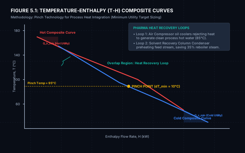
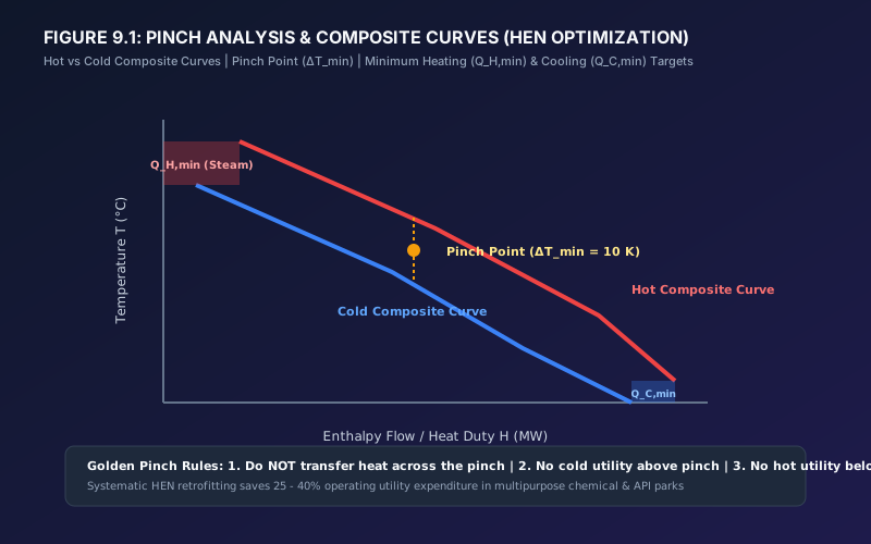
By combining all hot streams into a single cumulative heat flow vector and all cold streams into another, engineers construct the Temperature-Enthalpy () Composite Curves:
- Hot Composite Curve: Represents the total heat available from all process cooling duties across the temperature range.
- Cold Composite Curve: Represents the total heat demanded by all process heating duties across the temperature range.
When plotted together on a diagram, the curves are shifted horizontally until they reach a designated Minimum Temperature Approach ().
Temperature (T)
     ^
     |         / Hot Composite Curve (Heat Available)
     |        /
     |       /| <--- Overlap Zone: Feasible Process-to-Process Heat Recovery
     |      / |
     |     /  |        / Cold Composite Curve (Heat Required)
     |    /   |       /
     |   /    * <--->*   <--- PINCH POINT (dT_min)
     |  /             /
     | /             /
     |/             /  <--- Unmatched Cold End: Minimum Hot Utility (Q_H,min)
     +------------------------------------------------------------> Enthalpy (H)
       <-- Unmatched Hot End: Minimum Cold Utility (Q_C,min) -->
- The Overlap Region: Represents the maximum thermodynamically feasible Process-to-Process Heat Exchange ().
- The Cold Utility Deficit (): The hot composite curve extends beyond the cold curve at the low-temperature end, dictating the minimum external cooling duty (cooling tower or chilled water).
- The Hot Utility Deficit (): The cold composite curve extends beyond the hot curve at the high-temperature end, dictating the minimum external heating duty (steam or hot water).
# C. The Pinch Temperature ()
The point of closest approach () is the Pinch Point. The pinch divides the entire manufacturing facility into two thermodynamically distinct, independent thermodynamic systems:
- Above the Pinch (): Acts as a net Heat Sink. It demands heat from the outside world () but cannot reject any heat.
- Below the Pinch (): Acts as a net Heat Source. It has excess heat that must be rejected to cold utilities () but cannot absorb external heat.
# 2. The Three Golden Rules of Pinch Analysis
Pinch analysis provides three non-negotiable rules for process and utility engineers. Violating any of these rules introduces double energy penalties:
+=======================================================================================+
|                              THE THREE PINCH GOLDEN RULES                             |
+=======================================================================================+
| 1. DO NOT TRANSFER HEAT ACROSS THE PINCH:                                             |
|    Transferring heat from above the pinch to below the pinch increases BOTH hot      |
|    utility demand (steam) and cold utility demand (cooling water) by exactly that     |
|    amount! (A 100 kW cross-pinch transfer wastes 100 kW steam AND 100 kW cooling).    |
|                                                                                       |
| 2. DO NOT USE COLD UTILITIES ABOVE THE PINCH:                                         |
|    Cooling a stream above the pinch with cooling water robs heat from the process     |
|    heat sink, requiring an identical increase in boiler steam to compensate.          |
|                                                                                       |
| 3. DO NOT USE HOT UTILITIES BELOW THE PINCH:                                          |
|    Heating a stream below the pinch with steam adds unnecessary thermal energy into   |
|    a zone that already has a heat surplus, overloading cooling towers and chillers.   |
+=======================================================================================+
# The Cost of Violating the Pinch:
If an engineer transfers heat across the pinch:
A single improper piping tie-in transferring across the pinch wastes of steam PLUS of chilled water power, costing a manufacturing site over ₹35 Lakhs ($42,000 USD) every single year in redundant utility billing.
# 3. The Grand Composite Curve (GCC) & Utility Selection
While the Composite Curves determine overall heating and cooling targets, the Grand Composite Curve (GCC) plots net process heat deficit and surplus as a function of shifted temperature ( for hot streams; for cold streams):
Shifted Temp (T*)
       ^
       |        \            / Net Heating Deficit (Steam Required)
       |         \          /
       |          \        /
       |           \      /
  T*_pinch ---------> \  /  <--- PINCH POINT (Net Enthalpy = 0)
       |               \/
       |               /\
       |              /  \
       |             /    \  <--- Net Cooling Surplus (Cooling Water / Chilled Water)
       |            /      \
       +--------------------------------------------> Net Enthalpy (H_net)
# Utility Sizing & Temperature Level Matching:
The GCC enables process engineers to match specific industrial utilities to the exact thermodynamic temperature level required, avoiding high-grade energy destruction:
- High-Pressure Steam (10 bar g, 185°C): Reserved exclusively for high-temperature distillation reboilers and thermal fluid heaters.
- Low-Pressure Steam (3 bar g, 143°C): Used for bulk process preheating and evaporation.
- Waste Heat Hot Water (60°C - 80°C): Sourced from air compressors and vacuum pumps to supply cleanroom AHU pre-heat coils.
- Cooling Tower Water (32°C supply): Used for initial product cooling and condenser knockdown above 40°C.
- Chilled Water (7°C supply): Reserved for low-temperature condensation and crystallization below 30°C.
- Low-Temperature Glycol / Brine (-15°C to -25°C): Confined strictly to sub-ambient solvent freezing, cryogenic API syntheses, and VOC vent recovery.
# 4. The Problem Table Algorithm (Heat Cascade) & 4-Stream Worked Numerical Case Study
While graphical composite curves provide exceptional visual insight, industrial Heat Exchanger Network (HEN) design relies on the analytical Problem Table Algorithm (Heat Cascade) developed by Bodo Linnhoff. This algorithm computes exact hot utility demand (), cold utility demand (), and precise pinch temperatures without drawing errors.
# Problem Statement:
An API synthesis unit operates 2 hot process streams and 2 cold process streams. The chosen Minimum Temperature Approach is .
# Stream Data Table:
| Stream | Type | () | () | () | () |
|---|---|---|---|---|---|
| H1 | Hot | ||||
| H2 | Hot | ||||
| C1 | Cold | ||||
| C2 | Cold |
- Total Heat Available from Hot Streams: .
- Total Heat Demanded by Cold Streams: .
- Un-integrated baseline utility consumption: steam cooling water .
# Step 1: Interval Temperature Shifting
To enforce the approach throughout the network, hot stream temperatures are shifted down by and cold stream temperatures are shifted up by :
- : shifts to
- : shifts to
- : shifts to
- : shifts to
Rank-ordering the shifted boundary temperatures from highest to lowest yields 6 discrete temperature levels:
# Step 2: Heat Cascade Algorithm & Pinch Identification
Evaluating the enthalpy balance across each temperature interval ():
| Interval | Shifted Temp Range | Interval | Active Streams | Net | Interval Energy Balance () |
|---|---|---|---|---|---|
| 1 | H1 () | (Heat Surplus) | |||
| 2 | H1 (), H2 (), C2 () | (Heat Surplus) | |||
| 3 | H1 (), H2 (), C1 (), C2 () | (Heat Deficit) | |||
| 4 | H1 (), H2 (), C1 () | (Heat Surplus) | |||
| 5 | H2 (), C1 () | (Heat Deficit) |
Cascading cumulative heat downward assuming zero initial external hot utility ():
- Heat cascaded into Interval 1:
- After Interval 1:
- After Interval 2:
- After Interval 3: Maximum Cumulative Heat Deficit!
- After Interval 4:
- After Interval 5:
To ensure thermodynamic feasibility (no negative heat transfers), the cascade must be primed with an external heat input equal to the largest deficit:
- Minimum Hot Utility (Steam):
- Minimum Cold Utility (Cooling Water):
- Pinch Temperature Location: The zero-heat flux boundary occurs between Interval 2 and 3:
- Shifted Pinch Temperature:
- Hot Stream Pinch Temperature:
- Cold Stream Pinch Temperature:
# Step 3: Verified Energy & Carbon Reduction
- Baseline Steam Consumption: Pinch Target: ( Steam Reduction!)
- Baseline Cooling Water Duty: Pinch Target: ( Cooling Water Reduction!)
- Internal Heat Recovery: recovered directly within the process network!
# 5. Heat Exchanger Network (HEN) Synthesis & Sizing at the Pinch (The -Rules)
Placing heat exchangers at the pinch requires following strict -Rules to prevent temperature crossovers and preserve :
                      PINCH MATCHING FEASIBILITY CRITERIA
       ABOVE THE PINCH (Net Heat Sink)            BELOW THE PINCH (Net Heat Source)
     ─────────────────────────────────          ─────────────────────────────────
             CP_cold >= CP_hot                          CP_hot >= CP_cold
     Stream temperatures diverge moving         Stream temperatures diverge moving
     away from the pinch (ΔT expands).          away from the pinch (ΔT expands).
# Stream Splitting Rules:
- Above the Pinch: If an engineer must match a hot stream with a cold stream where , matching them directly will cause the temperature difference to narrow below or even crossover. The hot stream must be split into parallel branches so that .
- Below the Pinch: Conversely, if , the cold stream must be split into parallel branches so that .
- Number of Exchanger Units ():
The minimum number of units required to achieve maximum energy recovery is governed by Euler's network theorem:
# 6. The Pharmaceutical Dilemma: Why Classical Pinch Fails in Batch Plants
Classical Pinch Analysis was formulated for massive, steady-state chemical petrochemical plants (such as ethylene crackers and crude oil refineries) where streams run continuously 24 hours a day, 365 days a year.
When process engineers attempt to apply standard continuous pinch software (e.g., classic Aspen Energy Analyzer) to pharmaceutical batch manufacturing, the exercise frequently fails due to five distinct industry realities:
# A. The Non-Contemporaneity Barrier (Time Dependence)
In a batch API synthesis suite, heating and cooling demands are intermittent and non-simultaneous:
- Reactor R-101 requires of cooling to arrest an exothermic addition between 02:00 and 04:00.
- Distillation Column C-201 requires of reboiler heating between 08:00 and 12:00.
- Clean-In-Place (CIP) skid requires of hot water preheating between 16:00 and 17:30.
Because the hot stream and the cold stream do not exist at the same instant in time, direct process-to-process heat exchange is physically impossible without thermal storage buffer capacity.
# B. Strict cGMP Validation & Cross-Contamination Barriers
In pharmaceutical manufacturing, regulatory compliance (US FDA 21 CFR Part 211, EU GMP Annex 1, and ISPE Baseline Guides) supersedes thermal efficiency:
- Forbidden Direct Fluid Pairing: An engineer cannot exchange heat directly between an untreated chemical reaction mother liquor and a Water for Injection (WFI) loop. A tube rupture would cause catastrophic product adulteration.
- Sanitary Isolation Loops: Heat recovery must utilize intermediate, closed-loop, decoupled fluid loops (e.g., pressurized USP clean water or USP Propylene Glycol circuits) monitored continuously by online conductivity, TOC, and differential pressure sensors.
- Drainability & Cleanability: Heat exchangers in contact with product streams must be sanitary grade (ASME BPE compliant, 316L electropolished to , fully drainable, zero dead-legs).
# C. Multi-Product Campaign Flexibility & Recipe Variations
Unlike dedicated petrochemical units, pharmaceutical multi-purpose synthesis blocks produce different API molecules in rotating campaigns throughout the year:
- Campaign A (Oncology API): Low-temperature syntheses with heavy refrigeration and vacuum drying.
- Campaign B (Antibiotic Intermediate): High-temperature reflux boiling and high-volume aqueous extraction.
- A rigid heat exchanger network optimized strictly for Campaign A will be completely misaligned for Campaign B.
# D. Variable Rheology, Slurries, and Severe Fouling
During reaction mass cooling, precipitation, and crystallization, fluid viscosity can skyrocket by orders of magnitude (from to ), causing the overall heat transfer coefficient () to collapse from to under . Static pinch models that assume constant -values severely undersize heat exchange areas.
# 7. How Artificial Intelligence & Machine Learning Revolutionize Pinch Analysis
Artificial Intelligence, Machine Learning, and Industrial IoT (IIoT) transform Pinch Analysis from an academic, static calculation into an autonomous, dynamic, schedule-aware energy optimization engine.
+---------------------------------------------------------------------------------------+
|                       THE 5 PILLARS OF AI-DRIVEN PINCH IN PHARMA                      |
+---------------------------------------------------------------------------------------+
|                                                                                       |
|   [1. Automated Stream Mining] ----> Ingests SCADA/MES data, eBMRs, and P&IDs to     |
|                                      auto-extract dynamic (m * Cp * dT) intervals.    |
|                                                                                       |
|   [2. Dynamic Time-Slice Batch Pinch] -> Optimizes Thermal Energy Storage (TES)       |
|                                          charge/discharge across non-overlapping runs.|
|                                                                                       |
|   [3. Graph Neural Networks (GNN)] -> Synthesizes cGMP-compliant HEN topologies with  |
|                                       forbidden match isolation and pipe routing.     |
|                                                                                       |
|   [4. Physics-Informed Neural Networks] -> Millisecond real-time dT_min optimization  |
|                                            balancing CAPEX vs OPEX under weather shifts|
|                                                                                       |
|   [5. Predictive Fouling & Digital Twin] -> Forecasts U-value decay in condensers and|
|                                             schedules predictive CIP before pinch loss|
+---------------------------------------------------------------------------------------+
# Pillar 1: Automated Stream Mining & Data Reconciliation via NLP and Sensor AI
The Traditional Bottleneck: Historically, conducting a pinch analysis on a 50-reactor API plant required teams of energy consultants spending 3 to 6 months manually reviewing P&IDs, walking utility pipe bridges, and extracting temperature and mass flow data from batch records. By the time the pinch report was delivered, plant recipes had changed and the data was obsolete.
The AI Solution:
- Large Language Models (LLMs) & P&ID Vision Models: AI agents ingest digital P&IDs, process flow diagrams (PFDs), and electronic Batch Manufacturing Records (eBMRs) to automatically classify every process step into heating, cooling, condensing, or boiling duties.
- Automated Historian Mining: The AI connects directly to plant data historians (OSIsoft PI, Aspen InfoPlus.21, Wonderware) and SCADA systems. It processes millions of time-series sensor points (flow meters, PT100 temperature transmitters, jacket control valve positions) and extracts dynamic enthalpy intervals:
- Gross Error Detection (GED) & Data Reconciliation: Neural network autoencoders detect sensor drift, calibrate misread flow meters, and ensure that stream energy and mass balances satisfy First-Law conservation () before running pinch calculations.
# Pillar 2: Dynamic Time-Slice Batch Pinch & Thermal Energy Storage (TES) Optimization
To solve the non-contemporaneity problem, AI models apply Dynamic Multi-Period Pinch Analysis combined with Thermal Energy Storage (TES) buffer optimization.
- Time-Slicing Decomposition:
The AI breaks the 24-hour manufacturing schedule into discrete dynamic time intervals (). Within each time slice, an instantaneous Pinch Analysis is calculated. - Thermal Storage (TES) Integration:
When heat surplus occurs in Time Slice 1 () and heat deficit occurs in Time Slice 3 (), direct heat transfer is impossible.
The AI models a stratified water or thermal oil buffer tank:- Stored Thermal Energy:
- Deep Reinforcement Learning (DRL) Scheduling:
A Deep Q-Network (DQN) or Proximal Policy Optimization (PPO) agent acts as a virtual energy scheduler:- State Vector: Current reactor states, scheduled future batch steps, ambient temperature, utility pricing (peak vs. off-peak grid tariffs), and TES tank state-of-charge ().
- Action Space: Modulate charging/discharging flow rates into thermal storage tanks; advance or delay non-critical wash steps by 15-30 minutes to maximize concurrent overlap.
- Reward Function: Minimize net imported steam () and electrical chiller power () while penalizing batch cycle delays.
# Pillar 3: cGMP-Constrained Heat Exchanger Network (HEN) Synthesis using Graph Neural Networks (GNNs)
Designing an industrial Heat Exchanger Network (HEN) is an NP-hard Mixed-Integer Non-Linear Programming (MINLP) problem. In pharma, the network must satisfy dozens of regulatory and physical layout constraints.
How GNNs and Evolutionary AI Solve HEN Synthesis:
- Graph Representation: The chemical plant is modeled as a directed graph , where nodes () represent process streams, utility headers, and intermediate buffer loops, while edges () represent potential heat exchanger matches and piping runs.
- Regulatory Masking (Enforcing cGMP): The AI applies hard masking matrices disallowing any forbidden edges:
- Pipe Run & Spatial Constraints: Using physical 3D plant laser scan coordinates, the GNN penalizes exchanger matches between streams located on opposite sides of a 200-meter plant, preventing excessive pipe CAPEX and pumping head losses.
- Multi-Objective Optimization: Evaluates the Pareto frontier between CAPEX (number of exchangers, surface area , exotic alloys like Hastelloy C-22 or Glass-Lined Steel) and OPEX (annual steam and chilled water savings):
# Pillar 4: Physics-Informed Neural Networks (PINNs) for Real-Time Targeting
The selection of the Minimum Temperature Approach () is the single most critical decision in pinch design:
- Small (e.g., 5°C): Maximizes heat recovery, drastically cutting steam and cooling water, but requires massive heat exchanger surface areas (), exploding CAPEX.
- Large (e.g., 20°C): Reduces heat exchanger sizes and costs, but leaves huge amounts of waste heat unrecovered, increasing annual utility bills.
In reality, the optimal is not static: it fluctuates daily based on cooling tower wet-bulb temperatures (summer vs. winter), volatile fuel/steam costs, and fluctuating factory production throughput.
The PINN Advantage:
- Classical numerical MINLP solvers require 20 to 60 minutes to converge a complete plant model, making them useless for real-time control.
- Physics-Informed Neural Networks (PINNs) embed thermodynamic governing equations (Fourier's law of conduction, LMTD formulations, energy balances) directly into the neural network's loss function:
- The trained PINN model evaluates the optimal and utility valve split in under 5 milliseconds, enabling continuous, real-time supervisory control via the plant Distributed Control System (DCS).
# Pillar 5: Predictive Fouling Tracking & Dynamic Pinch Adaptation
In pharmaceutical condensers, crystallizers, and distillation reboilers, thermal performance degrades over time due to organic scale deposition, resin polymerisation, and bio-fouling.
- The Problem: When heat exchanger overall heat transfer coefficients () drop:
The actual approach temperature increases, driving the process away from the pinch target and silently forcing backup steam and chilled water valves to open.
- AI Predictive Fouling Engine:
- Recurrent Neural Networks (LSTM) and Temporal Convolutional Networks (TCN) analyze temperature and pressure drop profiles across all heat recovery exchangers.
- Predicts the exact trajectory of fouling resistance days in advance.
- Automatically calculates the economic threshold where the utility cost of thermal degradation exceeds the cost of a CIP cycle:
- Schedules automated CIP cleanings during planned recipe changeovers, ensuring heat recovery exchangers maintain near-design efficiency year-round.
# 8. Classical vs. AI-Driven Smart Pinch: Technical Comparison Matrix
| Engineering Dimension | Classical Pinch Analysis (Manual / Static) | AI-Driven Dynamic Pinch (Smart Digital Twin) |
|---|---|---|
| Operational Paradigm | Assumes 24/7 continuous steady-state operation. | Fully dynamic; models asynchronous batch recipes and time-slices. |
| Data Ingestion | 3 to 6 months of manual P&ID reviews and Excel data entry. | Automated in real-time via SCADA, PI Historian, and eBMR ingestion. |
| Time-Dependence & Non-Contemporaneity | Fails completely. Cannot match streams running at different hours. | Solved. Uses Reinforcement Learning to optimize Thermal Storage (TES). |
| cGMP & Cross-Contamination | Must be checked manually by engineers after network design. | Built-in constraint masking prevents any forbidden regulatory pairings. |
| Network Synthesis Method | Heuristic grid diagrams; manual stream splitting. | Graph Neural Networks (GNNs) evaluate millions of topologies. |
| Optimal Selection | Fixed static value chosen once during initial plant design. | Real-time PINN optimization adapting to weather and utility costs. |
| Fouling & Aging Handling | Fixed safety fouling factor () added during sizing. | Real-time tracking of with predictive CIP scheduling. |
| Typical Energy Savings in Batch Pharma | (Limited to continuous utility systems). | across entire manufacturing complex. |
| Implementation Payback Period | 2.5 to 5.0 years (due to oversized heat exchangers). | 9 to 18 months (optimized sizing and minimal repiping). |
# 9. Five Comprehensive Industrial Worked Examples
# Worked Example 1: Air Compressor Waste Heat Recovery for Clean-In-Place (CIP) Water (Continuous Utility Pinch)
# Problem Statement:
A biopharmaceutical facility operates three oil-free rotary screw utility air compressors supplying sterile clean air. The compressors run continuously, drawing of total electrical power. Under full load, of this electrical input () is converted into heat absorbed by the compressor cooling oil circuit and rejected to an outdoor dry cooler.
Concurrently, the manufacturing building requires of continuous Purified Water (PW) preheated from ambient () to for sanitization and Clean-In-Place (CIP) make-up, currently heated by utility steam.
# Thermodynamic Stream Data:
- Hot Stream (Compressor Oil): , , ,
- Cold Stream (Purified Water): (), , ,
# The Pinch Solution:
Selecting :
- Maximum achievable water preheat temperature from compressor oil:
- Actual heat exchanged limited by available hot stream duty:
- Water temperature leaving recovery heat exchanger:
- Residual steam heating required:
# Financial & Environmental Results:
- Steam Reduction: ( of steam at ).
- Annual Operating Hours: .
- Annual Energy Saved: ().
- Annual Cost Savings (Steam @ ₹2,200 / Ton): **₹79.5 Lakhs / year (34,000 USD).
- Simple Payback Period: 4.0 Months!
# Worked Example 2: Solvent Recovery Column Reboiler & Condenser Integration
# Problem Statement:
An API synthesis unit runs a continuous binary solvent recovery column reclaiming Ethyl Acetate from spent process liquors.
- Column Reboiler: Demands of thermal duty from steam to boil bottom liquid at .
- Column Overhead Condenser: Rejects of latent heat into cooling water condensing vapor at .
Because the condenser temperature () is below the reboiler temperature (), direct internal process heat recovery is impossible without work input (negative driving force).
# The Pinch Solution (Inter-Unit Integration):
Pinch analysis revealed a nearby multi-effect vacuum evaporation unit concentrating an aqueous mother liquor stream at a reduced pressure of , where the boiling temperature is .
[Solvent Recovery Column]                               [Vacuum Crystallizer / Evaporator]
Top Vapor: 78°C (580 kW)                                Operating Temp: 65°C
        |                                                              |
        +=========> [Integrated Shell-and-Tube Exchanger] <===========+
                     dT_driving = 78°C - 65°C = 13°C (Feasible!)
                     Condenses Solvent Vapor ---> Boils Mother Liquor
- Hot Stream: Ethyl acetate vapor at condensing to liquid at ().
- Cold Stream: Aqueous solution at boiling at under vacuum ().
- Driving Force: .
# Financial & Environmental Results:
- Steam Saved on Evaporator: of LP steam completely eliminated.
- Cooling Water Saved on Condenser: ( circulation load removed from cooling tower).
- Annual Cost Savings: ₹68.4 Lakhs / year ($82,500 USD).
- Payback Period: 6.5 Months.
# Worked Example 3 (AI Case Study): Multi-Period Batch Pinch with DRL-Controlled Thermal Storage (TES)
# Problem Statement:
A modern multi-product API block operates four batch synthesis reactors. The reactors execute non-synchronous hydrogenation, distillation, and crystallization recipes:
- Intermittent Waste Heat Sinks: Three vacuum solvent condensers periodically reject a combined of latent heat at into cooling tower water for per batch.
- Intermittent Heat Demands: 3 hours after distillation concludes, the reactors undergo cleaning, requiring of heating to bring cold WFI () to for a wash cycle.
- Under standard operation, steam and cooling towers supply of these loads because the operations never occur simultaneously.
# The AI Pinch Solution:
The engineering team deployed an AI-Driven Thermal Energy Storage (TES) Pinch Architecture:
[Reactor Solvent Condensers] (82°C Waste Heat)
             |
             v (During Distillation Cycle: 02:00 - 04:30)
+-------------------------------------------------------------+
|    STRATIFIED PRESSURIZED WATER THERMAL STORAGE TANK (TES)  |
|            Volume: 25 m³ | Insulated Polyurethane           |
|            Hot Zone: 78°C   |   Cold Return: 35°C           |
+-------------------------------------------------------------+
             |
             v (Discharged 3 Hours Later: 07:30 - 09:30)
[WFI Pre-Heating Skid for CIP Cycle] (Heats 20°C -> 75°C)
- Reinforcement Learning Agent (PPO Algorithm):
- Reads plant production schedules from SAP MES 24 hours in advance.
- Modulates variable-speed charging pumps to capture of condenser heat into a vertical stratified thermal buffer vessel, maintaining an internal thermocline ( top layer, bottom layer).
- Three hours later, when the CIP wash cycle initiates, the RL agent discharges the stored hot water through a dedicated plate-and-frame exchanger, preheating the incoming WFI to before trim steam raises it to .
- Autonomous Recipe Coordination:
- If two reactors finish distillation simultaneously, the AI slightly adjusts the feed pump rate on Reactor 2 by , spreading the heat rejection profile evenly to prevent TES tank thermal overflow.
# Measured Plant Performance:
- Condenser Heat Captured: per batch.
- Peak Boiler Steam Demand Reduction: reduction in peak plant steam draw, preventing boiler trips during simultaneous morning recipe starts.
- Annual Steam Savings: (₹40.0 Lakhs / year).
- Chiller / Cooling Tower Power Saved: (₹11.6 Lakhs / year).
- Total Annual Net Benefit: ₹51.6 Lakhs / year ($62,000 USD/year).
- System Payback (Tank + Pumps + AI Controller): 14 Months.
# Worked Example 4 (AI Case Study): Graph Neural Network (GNN) Synthesis of a cGMP-Compliant Decoupled HEN
# Problem Statement:
An API site installed a centralized solvent recovery building with three packed distillation columns recovering Dichloromethane (DCM), Isopropanol (IPA), and Toluene from contaminated multi-stream waste drums.
- Across the three columns, there were 6 hot streams (overhead vapor condensers and bottoms product coolers) and 5 cold streams (cold feed preheaters and reboilers).
- The combinatorial space of potential heat exchanger matches was over configurations.
- Crucially, the plant had strict FDA cross-contamination restrictions:
- Toluene and DCM streams could not share an exchanger shell due to toxic reactive hazard risks.
- Product streams could not connect directly across different product registration lines.
# The AI Graph Neural Network (GNN) Architecture:
The team deployed an Evolutionary Graph Neural Network:
- Graph Encoding: Streams were represented as feature vectors containing temperature, mass heat capacity (), corrosivity index, and cGMP barrier classification.
- Masked Topology Search: The GNN evaluated topologies per minute while mathematically masking forbidden pairings to zero probability.
- Decoupled Closed Thermal Loop Solution:
Instead of direct complex stream-to-stream cross-piping, the GNN identified an optimal Decoupled Closed Pressurized Water Thermal Loop (CWTL) operating between and :
[IPA Column Condenser (85°C)] ---> Yields 310 kW  ---+
                                                     |---> [Decoupled Intermediate Water Loop]
[Toluene Bottoms Cooler (105°C)] -> Yields 240 kW ---+     Operating at 3.0 bar g (No Boiling)
                                                                       |
                                                                       v
[DCM Feed Preheater (Preheats 22°C -> 48°C)] <-------------------------+ (Absorbs 210 kW)
[IPA Feed Preheater (Preheats 25°C -> 72°C)] <-------------------------+ (Absorbs 340 kW)
# Engineering & Financial Outcome:
- Total Energy Recycled: continuous thermal duty.
- cGMP Compliance: Zero risk of cross-contamination; intermediate water loop pressure is maintained higher than solvent streams, ensuring any hypothetical pinhole leak causes clean water ingress rather than toxic solvent mixing.
- Annual Steam & Chilled Water Savings: **₹82.5 Lakhs / year (94,000 USD).
- Simple Payback: 11.3 Months.
# Worked Example 5 (AI Case Study): AI Digital Twin for Dynamic Multi-Utility Header Dispatch
# Problem Statement:
A commercial sterile manufacturing plant operates three utility refrigeration levels:
- Tower Cooling Water (CW): supply (Lowest cost: ₹0.40 / kWh-th).
- Chilled Water (CHW): supply (Medium cost: ₹2.10 / kWh-th).
- Low-Temperature Brine (BRN): supply (High cost: ₹5.80 / kWh-th).
Process operators routinely used the lowest-temperature utility ( brine) for tasks that could be handled by chilled water or even cooling tower water, simply because "it cools the batch faster." This thermal destruction overloaded the refrigeration compressors, causing frequent electrical peak-demand penalty charges.
# The AI Solution:
A Physics-Informed Digital Twin was integrated with the plant Yokogawa DCS:
- The AI continuously monitors reactor batch step progress, ambient wet-bulb temperature, and reactor jacket heat transfer dynamics.
- Dynamic Three-Stage Utility Switching:
When cooling an API reaction mass from to :- Stage 1 (): AI routes Cooling Water (). Brine and chilled water valves are locked shut.
- Stage 2 (): AI smoothly shifts utility control to Chilled Water.
- Stage 3 (): AI enables Brine strictly for the final crystallization chilling.
# Financial & Operational Results:
- Brine Compressor Electrical Load Reduction: reduction in refrigeration power.
- Annual Electricity Saved: (₹71.2 Lakhs / year).
- Thermal Shock Prevention: Eliminated glass-lining delamination caused by premature injection of brine into hot reactor jackets.
- Payback Period: Immediate (Software & instrumentation optimization; zero major equipment CAPEX).
# 10. Step-by-Step Roadmap for Implementing AI Pinch in an Operating Facility
Process plants can implement an AI-driven Pinch Optimization program by following this systematic 6-step engineering protocol:
[Phase 1: Stream Identification & Digital Ingestion] (Week 1 - 4)
  - Connect AI ingestion pipeline to SCADA / PI Historian tags.
  - Parse P&IDs and eBMR recipes; establish validated enthalpy stream tables.
                         |
                         v
[Phase 2: Thermodynamic Pinch Targeting & GCC Analysis] (Week 5 - 8)
  - Run Problem Table Algorithm; generate Composite Curves and GCC.
  - Determine theoretical minimum utilities (Q_H,min and Q_C,min) across all products.
                         |
                         v
[Phase 3: Dynamic Batch Scheduling & TES Sizing] (Week 9 - 14)
  - Execute time-slice batch pinch analysis across rotating product campaigns.
  - Size Thermal Energy Storage (TES) buffer vessels and evaluate decoupled loop routing.
                         |
                         v
[Phase 4: cGMP Regulatory Screening & GNN Topology Optimization] (Week 15 - 18)
  - Apply regulatory constraint matrices (ISPE / FDA cross-contamination filters).
  - GNN generates Pareto-optimal HEN designs; select maximum NPV with sub-18 month payback.
                         |
                         v
[Phase 5: Turnkey Fabrication & Control Tie-In] (Week 19 - 28)
  - Install sanitary plate/shell-and-tube heat exchangers, buffer tanks, and VFD pumps.
  - Program DCS control blocks and train Deep Reinforcement Learning supervisory agent.
                         |
                         v
[Phase 6: Commissioning, Digital Twin Tracking & Predictive CIP] (Week 29+)
  - Commission automated heat recovery loops.
  - Activate real-time Digital Twin tracking overall heat transfer coefficients and fouling rates.
# 11. Key Mathematical Equations for Pinch Engineers
For process design calculations, engineers must utilize the following governing thermodynamic relationships:
| Formula Name | Mathematical Formulation | Engineering Application |
|---|---|---|
| Stream Enthalpy Flow | Heat load calculation for single-phase liquid/gas streams. | |
| Latent Stream Enthalpy | Heat load for condensing vapors or boiling reboilers. | |
| Interval Heat Deficit | Problem Table Algorithm interval energy cascade step. | |
| Log Mean Temp Difference | Sizing required heat exchanger surface area (). | |
| Minimum Surface Area | Sizing total plant heat exchanger surface area before design. | |
| TES Storage Capacity | Sizing stratified hot water buffer tanks for batch pinch. | |
| Fouling Rate Tracking | Real-time monitoring of exchanger degradation for predictive CIP. |
# 12. Interactive Engineering Calculators & Software Tools
To perform detailed thermal, hydraulic, and equipment sizing calculations related to this guide, utilize our interactive web suite:
- Heat Exchanger Design & LMTD Calculator →
Calculate Log Mean Temperature Difference (LMTD), overall heat transfer coefficients (), required surface area (), and pressure drop for shell-and-tube and plate heat exchangers. - Single Fluid System (TCU) Sizing Calculator →
Size closed-loop thermal control units (TCU), intermediate buffer heat exchangers, and expansion vessels for reactor heating and cooling. - Batch Reactor Scale-Up & Agitator Sizer →
Simulate reactor heat transfer rates (), jacket thermal duties, and scale-up parameters from laboratory to commercial vessels. - Reactor Shaft Mechanical Sizing Calculator →
Verify agitator shaft torque, deflection, and critical whirling speeds for jacketed synthesis reactors.
# 13. Applicable Engineering Standards & Regulatory Codes
All energy integration, heat exchanger installations, and thermal recovery loops designed in pharmaceutical facilities must comply with the following international engineering codes and cGMP regulations:
- ISO 50001:2018: Energy Management Systems — Requirements with Guidance for Use.
- VDI 4680: Pinch Analysis — Fundamentals and Industrial Applications (Verein Deutscher Ingenieure).
- US FDA 21 CFR Part 211.65 & 211.67: Equipment Design, Construction, and Cleaning in Pharmaceutical Manufacturing.
- ISPE Baseline Pharmaceutical Engineering Guide, Volume 4: Water and Steam Systems.
- ASME BPE-2024: Bioprocessing Equipment Standard (Sanitary Heat Exchanger Design, Drainability, and Electropolishing).
- ASME Boiler and Pressure Vessel Code (BPVC) Section VIII, Division 1 & 2: Rules for Construction of Pressure Vessels and Shell-and-Tube Heat Exchangers.
- TEMA Standards (Class R, C, and B): Tubular Exchanger Manufacturers Association Design Guidelines.
- EU GMP Annex 1: Manufacture of Sterile Medicinal Products (WFI Thermal Loop Integrity and Cross-Contamination Prevention).