# Numerical Methods & Process Optimization in Chemical Engineering: A Practical Python Guide

# Executive Summary & Engineering Scope

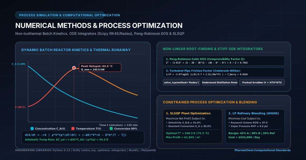
In industrial active pharmaceutical ingredient (API) manufacturing, specialty chemical processing, and refinery operations, process engineering models are rarely solvable using simple closed-form analytical equations. Realistic chemical systems involve non-linear thermodynamics (equations of state, non-ideal VLE activity models), stiff systems of coupled differential equations (transient reactor dynamics, heat transfer networks), and constrained multi-variable optimization problems (profit maximization, energy pinch analysis, utility scheduling).

Numerical methods and computational optimization provide process engineers with the mathematical engine needed to simulate, size, and optimize chemical plant operations.

This comprehensive technical guide covers:

Non-Linear Equations & Root-Finding: Solving non-ideal Equations of State (Peng-Robinson EOS), pipe friction factors (Colebrook-White), and distillation minimum reflux (Underwood equation).
Ordinary Differential Equations (ODEs) & Dynamic Systems: Simulating non-isothermal Plug Flow Reactors (PFR) and transient jacketed CSTR thermal runaway dynamics.
Mass Transfer & Separations: Numerical integration of Packed Scrubber Heights ( $H_{packed} = \text{HTU} \times \text{NTU}$ ) and multi-component stage calculations.
Kinetic Parameter Estimation: Non-linear least-squares fitting of experimental data to derive Arrhenius parameters ( $A, E_a$ ).
Constrained Continuous & Discrete Optimization: Plant profit optimization using SLSQP and refinery feedstock blending using Linear Programming (LP/HiGHS).

All sections feature mathematical derivations, process flow diagrams, and production-ready Python code snippets using numpy, scipy.optimize, scipy.integrate, and matplotlib.

# 1. Non-Linear Equations & Root-Finding in Process Engineering

# 1.1 Compressibility Factor ( $Z$ ) from Peng-Robinson Equation of State

Calculating molar volume ( $v$ ) or compressibility factor ( $Z = \frac{P v}{R T}$ ) for high-pressure gas streams requires solving cubic equations of state:

P = \frac{R T}{v - b} - \frac{a(T)}{v^2 + 2b v - b^2}

Expressed in dimensionless form for compressibility factor $Z$ :

f(Z) = Z^3 - (1 - B) Z^2 + (A - 2B - 3B^2) Z - (A B - B^2 - B^3) = 0

Where:

A = \frac{a(T) P}{R^2 T^2}, \quad B = \frac{b P}{R T}

# 1.2 Turbulent Pipe Friction Factor ( $f$ ) via Colebrook-White Equation

For turbulent flow in rough commercial steel pipes ( $Re > 4000$ ), the Darcy friction factor $f$ is implicitly defined by the non-linear Colebrook-White equation:

g(f) = \frac{1}{\sqrt{f}} + 2.0 \log_{10} \left( \frac{\varepsilon / D}{3.7} + \frac{2.51}{Re \sqrt{f}} \right) = 0

Where $\varepsilon / D$ is relative pipe roughness and $Re = \frac{\rho u D}{\mu}$ is the Reynolds number.

  +-----------------------------------------------------------------------------------+
  | NEWTON-RAPHSON ROOT-FINDING ALGORITHM FOR PROCESS EQUATIONS                       |
  +-----------------------------------------------------------------------------------+
  |                                                                                   |
  |   Initial Guess f_0 ──► Evaluate g(f_k) & g'(f_k) ──► f_{k+1} = f_k - g(f_k)/g'(f_k) |
  |                                                                 │                 |
  |                                                                 ▼                 |
  |   Converged? ◄──────────── Yes ◄─────────── |f_{k+1} - f_k| < 1e-8?               |
  |                                                                                   |
  +-----------------------------------------------------------------------------------+

# 1.3 Python Code: Peng-Robinson EOS & Colebrook-White Solvers

import numpy as np
from scipy.optimize import root_scalar

# --- 1. Peng-Robinson EOS Solver ---
def peng_robinson_z(P_bar, T_K, Tc_K, Pc_bar, omega):
    R = 8.314e-5  # bar*m^3/(mol*K)
    Tr = T_K / Tc_K
    kappa = 0.37464 + 1.54226 * omega - 0.26992 * (omega**2)
    alpha = (1 + kappa * (1 - np.sqrt(Tr)))**2
    
    a = 0.45724 * (R**2 * Tc_K**2 / Pc_bar) * alpha
    b = 0.07780 * (R * Tc_K / Pc_bar)
    
    A = (a * P_bar) / (R**2 * T_K**2)
    B = (b * P_bar) / (R * T_K)
    
    c2 = -(1 - B)
    c1 = A - 2*B - 3*(B**2)
    c0 = -(A*B - B**2 - B**3)
    
    f = lambda Z: Z**3 + c2*Z**2 + c1*Z + c0
    df = lambda Z: 3*Z**2 + 2*c2*Z + c1
    
    # Newton-Raphson iterations
    Z_curr = 1.0
    for i in range(100):
        Z_next = Z_curr - f(Z_curr) / df(Z_curr)
        if abs(Z_next - Z_curr) < 1e-8:
            break
        Z_curr = Z_next
        
    v_molar = (Z_next * R * T_K) / P_bar
    return Z_next, v_molar

# --- 2. Colebrook-White Friction Factor Solver ---
def colebrook_white_friction(Re, rel_roughness):
    # Haaland equation initial guess
    f_guess = 1.0 / (-1.8 * np.log10((rel_roughness / 3.7)**1.1 + 6.9 / Re))**2
    
    def g(f):
        return 1.0 / np.sqrt(f) + 2.0 * np.log10((rel_roughness / 3.7) + 2.51 / (Re * np.sqrt(f)))
        
    res = root_scalar(g, x0=f_guess, x1=f_guess*1.1, method='secant')
    return res.root

# Test Solvers
Z_val, v_mol = peng_robinson_z(50.0, 350.0, 305.3, 48.7, 0.099)  # Ethane
f_darcy = colebrook_white_friction(Re=250000, rel_roughness=0.00015)  # Steel pipe

print(f"Ethane Compressibility Factor Z : {Z_val:.5f} (Molar Vol: {v_mol*1e3:.3f} L/mol)")
print(f"Darcy Friction Factor (f)       : {f_darcy:.5f}")

# 2. ODE Systems & Transient Reactor Dynamics

# 2.1 Physical Problem: Transient Jacketed CSTR Thermal Runaway

Consider a continuous stirred-tank reactor (CSTR) conducting an exothermic first-order reaction $A \to B$ cooled by an external jacket:

                 Coolant Inlet (T_j0)
                          │
                          ▼
                  ┌───────────────┐
   Feed Stream    │  Jacketed     │   Product Stream
   F_0, C_A0, T_0 ├──► CSTR       ├──► F_0, C_A(t), T(t)
                  │  Volume V     │
                  └───────┬───────┘
                          │
                          ▼
                 Coolant Outlet (T_j)

The transient mass balance for species $A$ and energy balances for reactor fluid ( $T$ ) and cooling jacket ( $T_j$ ) are:

\frac{dC_A}{dt} = \frac{F_0}{V}(C_{A,0} - C_A) - k(T) C_A

\frac{dT}{dt} = \frac{F_0}{V}(T_0 - T) + \frac{(-\Delta H_{rxn})}{\rho C_p} k(T) C_A - \frac{U A_{heat}}{\rho V C_p}(T - T_j)

\frac{dT_j}{dt} = \frac{F_j}{V_j}(T_{j,in} - T_j) + \frac{U A_{heat}}{\rho_j V_j C_{pj}}(T - T_j)

Where $k(T) = A_{pre} \exp \left( -\frac{E_a}{R T} \right)$ .

# 2.2 Python Code: Dynamic CSTR Thermal Runaway & Emergency Cooling

import numpy as np
from scipy.integrate import solve_ivp

def cstr_transient_model(t, y, params):
    CA, T, Tj = y
    
    F0 = params['F0']        # m^3/s
    V = params['V']          # m^3
    CA0 = params['CA0']      # mol/m^3
    T0 = params['T0']        # K
    rho = params['rho']      # kg/m^3
    Cp = params['Cp']        # J/kg*K
    dH = params['dH']        # J/mol (Exothermic)
    U = params['U']          # W/m^2*K
    A_h = params['A_h']      # m^2
    Fj = params['Fj']        # Coolant flow m^3/s
    Vj = params['Vj']        # Jacket volume m^3
    Tjin = params['Tjin']    # Coolant inlet K
    rho_j = params['rho_j']  # Coolant density
    Cp_j = params['Cp_j']    # Coolant Cp
    A_pre = params['A_pre']  # 1/s
    Ea = params['Ea']        # J/mol
    R = 8.314
    
    k = A_pre * np.exp(-Ea / (R * T))
    
    dCA_dt = (F0 / V) * (CA0 - CA) - k * CA
    dT_dt = (F0 / V) * (T0 - T) + ((-dH) / (rho * Cp)) * k * CA - (U * A_h / (rho * V * Cp)) * (T - Tj)
    dTj_dt = (Fj / Vj) * (Tjin - Tj) + (U * A_h / (rho_j * Vj * Cp_j)) * (T - Tj)
    
    return [dCA_dt, dT_dt, dTj_dt]

# CSTR Operating Parameters
params = {
    'F0': 0.01, 'V': 2.0, 'CA0': 2000.0, 'T0': 300.0,
    'rho': 1000.0, 'Cp': 4184.0, 'dH': -90000.0,
    'U': 600.0, 'A_h': 8.0, 'Fj': 0.015, 'Vj': 0.5,
    'Tjin': 285.0, 'rho_j': 1000.0, 'Cp_j': 4184.0,
    'A_pre': 2.5e9, 'Ea': 68000.0
}

# Initial Steady State: CA = 450 mol/m^3, T = 345 K, Tj = 310 K
y0 = [450.0, 345.0, 310.0]
t_span = (0, 3600)  # 1 Hour dynamic simulation
t_eval = np.linspace(0, 3600, 360)

sol = solve_ivp(cstr_transient_model, t_span, y0, args=(params,), t_eval=t_eval, method='Radau')

print(f"Maximum Transient Peak Temperature : {np.max(sol.y[1]):.2f} K")
print(f"Final Steady-State Temperature      : {sol.y[1][-1]:.2f} K")

# 3. Mass Transfer & Separations (Scrubber Sizing & Underwood Equation)

# 3.1 Packed Scrubber Column Height Integration

Designing a packed gas absorption column for Acid Gas Scrubbing ( $\text{HCl}$ / $\text{NH}_3$ ) requires integrating the Height of a Transfer Unit (HTU) and Number of Transfer Units (NTU):

H_{packed} = \text{HTU} \times \text{NTU} = \left( \frac{G}{K_G a P} \right) \int_{y_{out}}^{y_{in}} \frac{dy}{y - y^*(x)}

Where $y^*(x) = m \cdot x$ represents gas-liquid equilibrium relationship.

# 3.2 Underwood Equation for Minimum Reflux Ratio ( $R_{min}$ )

In multi-component distillation shortcut design, the Underwood root $\theta$ lies between the relative volatilities of the light key (LK) and heavy key (HK) ( $1.0 < \theta < \alpha_{LK}$ ):

\sum_{i=1}^{n} \frac{\alpha_i \cdot z_{i,feed}}{\alpha_i - \theta} = 1 - q

Once $\theta$ is calculated, minimum reflux ratio $R_{min}$ is obtained via:

R_{min} + 1 = \sum_{i=1}^{n} \frac{\alpha_i \cdot x_{i,distillate}}{\alpha_i - \theta}

# 3.3 Python Code: Numerical Integration & Underwood Root Solver

import numpy as np
from scipy.integrate import quad
from scipy.optimize import root_scalar

# --- 1. Scrubber Height Numerical Integration ---
def integrate_scrubber_height(y_in, y_out, m_slope, G_mol_s, Ka_mol_m3_s):
    # Operating line: x(y) assuming pure liquid solvent feed (x_in = 0)
    L_over_G = 1.8 * m_slope  # 1.8x minimum L/G ratio
    
    def integrand(y):
        x = (y - y_out) / L_over_G
        y_eq = m_slope * x
        return 1.0 / (y - y_eq)
        
    NTU, _ = quad(integrand, y_out, y_in)
    HTU = G_mol_s / Ka_mol_m3_s
    H_packed = HTU * NTU
    return HTU, NTU, H_packed

# --- 2. Underwood Minimum Reflux Root Solver ---
def solve_underwood_rmin(alpha, z_feed, x_dist, q_factor):
    def underwood_eq(theta):
        return np.sum((alpha * z_feed) / (alpha - theta)) - (1.0 - q_factor)
        
    res = root_scalar(underwood_eq, bracket=[1.01, 2.09], method='brentq')
    theta_opt = res.root
    
    Rmin = np.sum((alpha * x_dist) / (alpha - theta_opt)) - 1.0
    return theta_opt, Rmin

# Test Mass Transfer Functions
HTU, NTU, H_scrubber = integrate_scrubber_height(y_in=0.08, y_out=0.001, m_slope=0.75, G_mol_s=25.0, Ka_mol_m3_s=3.2)
alpha_sys = np.array([4.0, 2.1, 1.0, 0.4])
z_sys = np.array([0.25, 0.35, 0.30, 0.10])
x_sys = np.array([0.41, 0.57, 0.02, 0.00])

theta_root, R_min = solve_underwood_rmin(alpha_sys, z_sys, x_sys, q_factor=1.0)

print(f"Scrubber Sizing Results : HTU = {HTU:.2f} m | NTU = {NTU:.2f} | Bed Height = {H_scrubber:.2f} m")
print(f"Underwood Root (theta) : {theta_root:.4f} | Minimum Reflux Ratio Rmin : {R_min:.2f}")

# 4. Kinetic Parameter Estimation & Curve Fitting

# 4.1 Parameter Estimation via Non-Linear Least Squares

Estimating Arrhenius rate parameters ( $A, E_a$ ) from experimental batch reactor concentration-time data requires minimizing the Sum of Squared Residuals (SSR):

S(A, E_a) = \sum_{i=1}^{N_{temps}} \sum_{j=1}^{N_{times}} \left( C_{A,exp}(t_j, T_i) - C_{A,pred}(t_j, T_i; A, E_a) \right)^2

# 4.2 Python Code: Kinetic Regression & Confidence Intervals

import numpy as np
from scipy.optimize import minimize
from scipy.integrate import solve_ivp

# Experimental Data (t in min, CA in kmol/m^3)
t_exp = np.array([0, 15, 30, 45, 60, 90, 120])
CA_310K = np.array([2.00, 1.68, 1.41, 1.19, 1.00, 0.71, 0.50])
CA_330K = np.array([2.00, 1.25, 0.78, 0.49, 0.31, 0.12, 0.05])

def fit_kinetics():
    def get_pred_CA(k, t_eval):
        sol = solve_ivp(lambda t, CA: -k * CA, (0, t_eval[-1]), [2.0], t_eval=t_eval)
        return sol.y[0]

    def objective(params):
        ln_A, Ea_kJ = params
        A = np.exp(ln_A)
        Ea = Ea_kJ * 1000.0
        R = 8.314
        
        k_310 = A * np.exp(-Ea / (R * 310.0)) * 60.0  # 1/min
        k_330 = A * np.exp(-Ea / (R * 330.0)) * 60.0
        
        pred_310 = get_pred_CA(k_310, t_exp)
        pred_330 = get_pred_CA(k_330, t_exp)
        
        ssr = np.sum((CA_310K - pred_310)**2) + np.sum((CA_330K - pred_330)**2)
        return ssr

    res = minimize(objective, [20.0, 55.0], method='L-BFGS-B', bounds=[(5, 35), (20, 120)])
    opt_A = np.exp(res.x[0])
    opt_Ea = res.x[1]
    
    return opt_A, opt_Ea, res.fun

A_opt, Ea_opt, ssr_val = fit_kinetics()
print(f"Pre-exponential Factor (A) : {A_opt:.3e} 1/s")
print(f"Activation Energy (Ea)     : {Ea_opt:.2f} kJ/mol")
print(f"Residual Sum of Squares    : {ssr_val:.6f}")

# 5. Constrained Continuous & Discrete Optimization

# 5.1 Multivariable Plant Profit Optimization (SLSQP)

Maximizing continuous chemical plant net profit subject to product purity ( $ge 92%$ ), minimum conversion ( $ge 85%$ ), and operating temperature limits ( $310\text{ K} \le T \le 385\text{ K}$ ):

J(T, \tau) = P_B \cdot C_B - P_A \cdot C_{A,0} - C_{utility}(T) - C_{capital}(\tau)

# 5.2 Refinery Feedstock Blending (Linear Programming / HiGHS)

Minimizing raw material costs for 3 intermediate blending streams subject to minimum Octane (RON $\ge 87.0$ ) and maximum Reid Vapor Pressure (RVP $\le 9.0\text{ psi}$ ).

# 5.3 Python Code: SLSQP Plant Profit & LP Refinery Blending

from scipy.optimize import minimize, linprog

# --- 1. SLSQP Process Optimization ---
def optimize_chemical_plant():
    CA0 = 2.0
    
    def profit_obj(x):
        T, tau = x
        k1 = 1.2e7 * np.exp(-55000 / (8.314 * T))
        k2 = 4.5e8 * np.exp(-70000 / (8.314 * T))
        
        CA = CA0 / (1 + k1 * tau)
        CB = (k1 * tau * CA) / (1 + k2 * tau)
        
        profit = (150.0 * CB) - (25.0 * CA0) - 0.05 * (T - 300)**1.5 - 0.8 * tau**1.2
        return -profit
        
    cons = [
        {'type': 'ineq', 'fun': lambda x: (1.2e7*np.exp(-55000/(8.314*x[0]))*x[1]*(CA0/(1+1.2e7*np.exp(-55000/(8.314*x[0]))*x[1]))/(1+4.5e8*np.exp(-70000/(8.314*x[0]))*x[1])) / (CA0 - (CA0/(1+1.2e7*np.exp(-55000/(8.314*x[0]))*x[1]))) - 0.92},
        {'type': 'ineq', 'fun': lambda x: 1 - (CA0/(1+1.2e7*np.exp(-55000/(8.314*x[0]))*x[1]))/CA0 - 0.85}
    ]
    
    res = minimize(profit_obj, [340.0, 30.0], method='SLSQP', bounds=[(310, 385), (5, 120)], constraints=cons)
    return res.x[0], res.x[1], -res.fun

# --- 2. LP Refinery Blending ---
def optimize_refinery_blend():
    c = [45.0, 52.0, 70.0]
    A_ub = [[9.0, 3.0, -11.0], [2.5, -1.0, -5.0]]
    b_ub = [0.0, 0.0]
    A_eq = [[1.0, 1.0, 1.0]]
    b_eq = [10000.0]
    bounds = [(0, 5000), (0, 4000), (0, 6000)]
    
    res = linprog(c, A_ub=A_ub, b_ub=b_ub, A_eq=A_eq, b_eq=b_eq, bounds=bounds, method='highs')
    return res.x, res.fun

opt_T, opt_tau, max_prof = optimize_chemical_plant()
blend_recipe, min_cost = optimize_refinery_blend()

print(f"Plant Optimization : T = {opt_T:.1f} K | tau = {opt_tau:.1f} min | Max Profit =  ${max_prof:.2f}/m^3") print(f"Refinery Blending : Naphtha A={blend_recipe[0]:.0f}, B={blend_recipe[1]:.0f}, Reformate={blend_recipe[2]:.0f} bbl/day | Cost =$ {min_cost:,.2f}/day")

# 6. Engineering Implementation Checklist for Process Modelers

Variable Normalization: Always scale decision variables with different orders of magnitude (e.g., Temperature $350\text{ K}$ vs Concentration $0.001\text{ mol/m}^3$ ) to optimize condition numbers.
Stiffness Management: Use implicit stiff integrators (method='Radau' or method='BDF') for non-isothermal runaway reactions or fast kinetic networks.
Physical Bounds: Enforce non-negative bounds ( $C_i \ge 0$ , $T \ge 273.15\text{ K}$ ) on state variables during numeric iterations.
Multi-Start Verification: Perform multi-start optimization initializations to confirm global optimality in non-convex search spaces.

# Applicable Engineering Standards & References

Fogler, H. S. Elements of Chemical Reaction Engineering (5th Edition, Prentice Hall).
Edgar, T. F., Himmelblau, D. M., & Lasdon, L. S. Optimization of Chemical Processes (McGraw-Hill).
Press, W. H., et al. Numerical Recipes: The Art of Scientific Computing (Cambridge University Press).
ISO 5167 / ASME MFC-3M: Measurement of Fluid Flow by Means of Pressure Differential Devices.