# Capital Allocation in Process Engineering: Evaluating & Selecting Between Competing CAPEX Projects via ROI, NPV, IRR, and Life-Cycle OPEX Analysis
# Executive Summary & Engineering Economics Context
In chemical processing plants, pharmaceutical API manufacturing facilities, and oil & gas refineries, process engineering leaders and site executives face a recurring strategic challenge: How to allocate limited Capital Expenditure (CAPEX) between mutually exclusive process improvement proposals?
When two engineering solutions solve the same operational problem—such as choosing between a low-CAPEX/high-OPEX conventional utility system versus a high-CAPEX/ultra-low-OPEX energy-efficient system—relying solely on upfront equipment purchase price leads to severe financial sub-optimization.
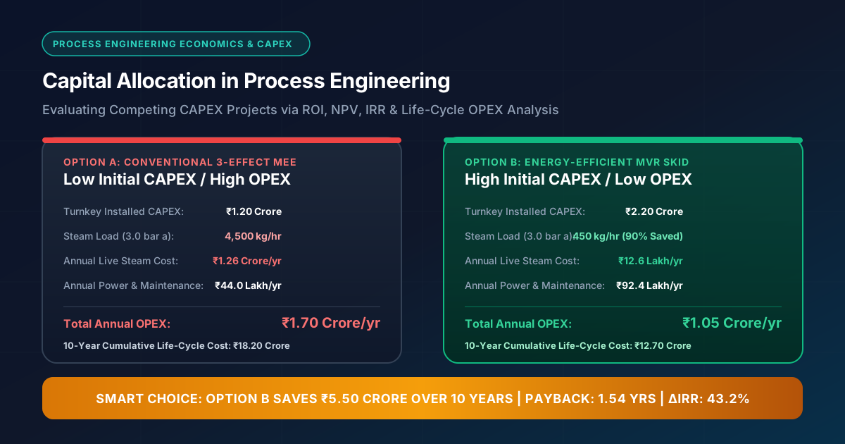
  THE CAPEX DECISION DILEMMA (UPFRONT COST VS LIFE-CYCLE VALUE)
  ┌────────────────────────────────────────────────────────────────────────────┐
  │ OPTION A: Low Initial CAPEX / High Annual OPEX                             │
  │ • Equipment Cost: ₹1.20 Crore | Annual OPEX: ₹1.70 Crore/yr                │
  │ • 10-Year Cumulative Life-Cycle Cost: ₹18.20 Crore                         │
  ├────────────────────────────────────────────────────────────────────────────┤
  │ OPTION B: High Initial CAPEX / Ultra-Low Annual OPEX (The Smart Choice)    │
  │ • Equipment Cost: ₹2.20 Crore | Annual OPEX: ₹1.05 Crore/yr                │
  │ • 10-Year Cumulative Life-Cycle Cost: ₹12.70 Crore                        │
  │ • 10-Year Net Life-Cycle OPEX Savings: ₹5.50 CRORE SAVED!                 │
  └────────────────────────────────────────────────────────────────────────────┘
Selecting the optimal investment requires a unified framework combining first-principles chemical engineering performance modeling with corporate financial metrics:
- Net Present Value (NPV): Accounting for time value of money.
- Internal Rate of Return (IRR): Comparing project return against the corporate hurdle rate (WACC).
- Incremental Return on Investment () and Discounted Payback Period (DPP).
- Life-Cycle Total Cost of Ownership (TCO) and Levelized Cost of Production (LCOP).
- Sensitivity & Risk Analysis: Stress-testing against utility price fluctuations (coal, gas, power tariffs), production volume variations, and plant downtime.
This technical guide provides process engineers, project managers, and financial executives with a rigorous quantitative methodology and a worked industrial case study for evaluating competing CAPEX proposals in Indian rupees (₹ in Crores & Lakhs).
# 1. Quantitative Financial & Engineering Evaluation Metrics
# 1.1 Net Present Value (NPV)
Net Present Value measures the net financial value generated by a project over its operating lifetime, discounted back to present value at the company's Weighted Average Cost of Capital (WACC or discount rate ):
Where:
- = Total initial installed capital expenditure in ₹ (Equipment + Civil + Piping + Electrical + C&I + Commissioning)
- = Net cash flow in year
- = Corporate discount rate / hurdle rate (typically for Indian process industries)
- = Asset economic life (typically 10 to 15 years)
- = Corporate tax rate (typically )
# 1.2 Internal Rate of Return (IRR) & Incremental IRR ()
The Internal Rate of Return (IRR) is the discount rate at which the project's equals zero:
When choosing between Option A (Low CAPEX) and Option B (High CAPEX), evaluate the Incremental IRR () on the additional capital spent ():
# 1.3 Discounted Payback Period (DPP) & Simple Payback
Simple Payback Period measures the time required to recover the initial CAPEX from non-discounted annual cash savings:
Discounted Payback Period (DPP) incorporates the time value of money and calculates the exact year where cumulative discounted cash flows equal initial CAPEX:
# 1.4 Life-Cycle Total Cost of Ownership (TCO)
Total Cost of Ownership evaluates the full financial burden over the asset lifecycle:
# 2. Worked Industrial Case Study: MEE vs. MVR Wastewater ZLD Skids
A 200 KL/day specialty chemical API plant must install a Zero Liquid Discharge (ZLD) effluent evaporation system to concentrate high-TDS wastewater.
Two technical options are proposed by engineering teams:
- Option A: Conventional Triple Effect Evaporator (MEE)
- Low initial equipment cost, but heavy steam consumption from the main utility boiler.
- Option B: Mechanical Vapor Recompression (MVR) Evaporator Skid
- High initial equipment cost, but uses an electric turbo-compressor to recompress vapor, eliminating of live steam consumption.
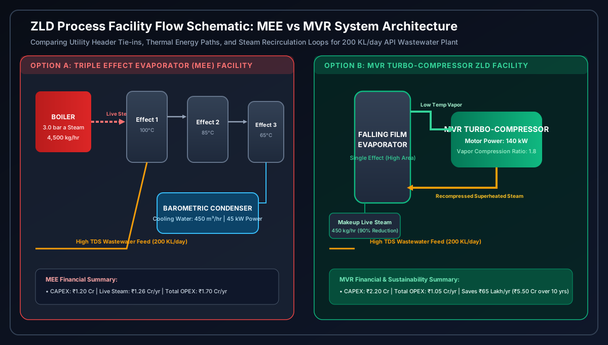
# Technical & Financial Parameters Comparison
| Technical & Financial Parameter | Option A: Triple Effect Evaporator (MEE) | Option B: Mechanical Vapor Recompression (MVR) | Delta / Operational Impact () |
|---|---|---|---|
| Turnkey Installed CAPEX | ₹1,20,00,000 (₹1.20 Cr) | ₹2,20,00,000 (₹2.20 Cr) | +₹1,00,00,000 (+₹1.00 Cr Additional Capital) |
| Live Steam Consumption (3.0 bar a) | 4,500 kg/hr (4.5 tonnes/hr) | 450 kg/hr (0.45 tonnes/hr) | -4,050 kg/hr (90% Live Steam Reduction) |
| Electricity Consumption | 45 kW | 140 kW | +95 kW (Higher Compressor Duty) |
| Annual Steam Cost (₹3,500/tonne, 8,000 h/yr) | ₹1,26,00,000 / yr (₹1.26 Cr/yr) | ₹12,60,000 / yr (₹12.6 Lakh/yr) | -₹1,13,40,000 / yr (-₹1.134 Cr/yr Steam Savings) |
| Annual Electricity Cost (₹8.0/kWh, 8,000 h/yr) | ₹28,80,000 / yr (₹28.8 Lakh/yr) | ₹70,40,000 / yr (₹70.4 Lakh/yr) | +₹41,60,000 / yr (+₹41.6 Lakh/yr Power Cost) |
| Annual Maintenance & Spares Cost | ₹15,20,000 / yr (₹15.2 Lakh/yr) | ₹22,00,000 / yr (₹22.0 Lakh/yr) | +₹6,80,000 / yr (+₹6.8 Lakh/yr Spares & SLA) |
| Total Annual Operating Cost (OPEX) | ₹1,70,00,000 / yr (₹1.70 Cr/yr) | ₹1,05,00,000 / yr (₹1.05 Cr/yr) | -₹65,00,000 / yr (₹65.0 Lakh/yr Net OPEX Savings) |
# Step-by-Step Financial Comparison
# 1. Annual Net OPEX Savings of Option B over Option A:
# 2. Incremental Initial CAPEX Required for Option B:
# 3. Simple Incremental Payback Period:
# 4. 10-Year Net Present Value (NPV) Comparison (At Hurdle Rate, Tax ):
- After-tax annual cash flow .
- Present Value Factor for 10 years at .
# 5. Incremental Internal Rate of Return ():
  10-YEAR CUMULATIVE LIFE-CYCLE COST COMPARISON (IN ₹ CRORES)

  Cost (₹ Crores)
   20.0 ┤                                        Option A (MEE): ₹18.20 Crore Total
   17.5 ┤                                 ┌───────┐
   15.0 ┤                          ┌──────┘       │
   12.5 ┤                   ┌──────┘              │  Option B (MVR): ₹12.70 Crore Total
   10.0 ┤            ┌──────┘       ┌─────────────┘ (SAVINGS: ₹5.50 CRORES Saved!)
    7.5 ┤     ┌──────┘       ┌──────┘
    5.0 ┤ ┌───┘       ┌──────┘
    2.5 ┼─┘───────────┘
    0.0 └─┬───┬───┬───┬───┬───┬───┬───┬───┬───┬───
         Y0  Y1  Y2  Y3  Y4  Y5  Y6  Y7  Y8  Y9 Y10
# 3. Engineering Risk Factors & Qualitative Decision Criteria
While financial metrics provide the core quantitative baseline, chemical process decisions must incorporate engineering risk criteria:
| Decision Criterion | Option A (Low CAPEX / High OPEX) | Option B (High CAPEX / Low OPEX) | Engineering Evaluation & Impact |
|---|---|---|---|
| Utility Dependency & Vulnerability | High dependency on boiler steam capacity (). | Operates primarily on grid/solar electricity (). | Option B reduces site steam header load, avoiding boiler expansion CAPEX. |
| Process Control & Automation | Manual/semi-automated steam valve throttling. | Fully automated PLC/SCADA compressor speed control. | Option B offers tighter temperature control and lower operator intervention. |
| Carbon Footprint & ESG (Scope 1 Emissions) | High direct emissions from steam generation (). | Low site emissions; eligible for green power purchasing. | Option B aligns with corporate net-zero targets and ESG reporting. |
| Maintenance & Asset Reliability | Low complexity; standard pumps and heat exchanger tubes. | High complexity; requires precision turbo-compressor maintenance. | Option A has lower specialized spare parts risk; Option B requires vendor SLA. |
| Future Expansion Scalability | Linear scaling required; high utility footprint. | Modular skid expansion; compact footprint. | Option B occupies less floor space in cleanroom/utility yards. |
# 4. A 5-Step CAPEX Selection Decision Matrix & Framework
To systematically evaluate competing CAPEX proposals in your engineering organization, follow this 5-step protocol:
  5-STEP CAPEX SELECTION PROTOCOL
  ┌──────────────────────────────────────────────────────────────────────────┐
  │ Step 1: DEFINE FULL LIFE-CYCLE BOUNDARIES                                │
  │         Include equipment purchase, installation, utilities, & maintenance│
  ├──────────────────────────────────────────────────────────────────────────┤
  │ Step 2: BUILD FIRST-PRINCIPLES ENERGY & MASS BALANCE MODELS               │
  │         Quantify utility consumption (steam, power, chilled water, N2).   │
  ├──────────────────────────────────────────────────────────────────────────┤
  │ Step 3: CALCULATE DISCOUNTED FINANCIAL METRICS (IN ₹ LAKHS / CRORES)     │
  │         Determine NPV, IRR, Incremental IRR, and Discounted Payback.       │
  ├──────────────────────────────────────────────────────────────────────────┤
  │ Step 4: STRESS-TEST WITH SENSITIVITY & MONTE CARLO SIMULATIONS          │
  │         Evaluate ±20% shifts in energy prices, production rate, & WACC.    │
  ├──────────────────────────────────────────────────────────────────────────┤
  │ Step 5: EXECUTE RISK & SAFETY GOVERNANCE SIGN-OFF                        │
  │         Verify HAZOP compatibility, MOC integrity, and OEB containment.   │
  └──────────────────────────────────────────────────────────────────────────┘
# 5. Summary & Strategic Recommendations
- Never Select Process Assets on Upfront Purchase Price Alone: In continuous and batch chemical/pharma plants, annual utility and maintenance OPEX typically exceeds initial CAPEX within 2 to 3 years.
- Use Incremental IRR () as the Primary Decision Metric: When evaluating a higher CAPEX option, ensure the additional capital yields an incremental IRR well above the company's cost of capital.
- Factor in Utility Header Capacity: Choosing energy-efficient skids (like MVR evaporators, monofluid TCUs, or heat-pump dryers) frees up boiler and chiller capacity for revenue-generating synthesis reactors.
Use our interactive Process Engineering Calculators & Sizing Tools to model energy balances, utility costs, and financial payback periods for your plant projects!
# Regulatory Standards & Financial References
- AACE International: Recommended Practice No. 18R-97 - Cost Estimate Classification System As Applied in Engineering, Procurement, and Construction for the Process Industries.
- Turton, R. et al.: Analysis, Synthesis, and Design of Chemical Processes (5th Edition, Prentice Hall).
- Peters, M.S., Timmerhaus, K.D., West, R.E.: Plant Design and Economics for Chemical Engineers (5th Edition, McGraw-Hill).
- ISPE: Baseline Pharmaceutical Engineering Guide Volume 3 - Commissioning and Qualification (2nd Edition).